Periodic Random Field Generation and Analysis
Generate periodic 1D/2D/3D Gaussian and non-Gaussian random fields with prescribed power spectra using Fourier-space filtering and prescribed Height Distribution. Includes tools for spectral analysis, autocorrelation, and statistical moments.
-
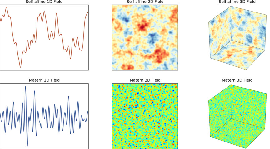
Self-affine (power-law) spectrum — controlled by Hurst exponent
$H \in [0, 1]$ -
Matérn covariance spectrum — controlled by smoothness parameter
$\nu > 0$ - Arbitrary PSD and PDF — Control both power spectrum and amplitude distribution (IAAFT)

-
Two generation modes:
-
noise=True: Filtered white noise (spectrum follows target on average) -
noise=False: Ideal spectrum with random phases (spectrum matches target exactly)
-
-
Analysis tools:
- Fast FFT-based autocorrelation (1D, 2D, N-D)
- Power spectral density computation
- Spectral moments (
$m_{00}$ ,$m_{20}$ ,$m_{02}$ ,$m_{40}$ ,$m_{04}$ , etc.) - Hurst exponent estimation
- RMS height, slope, curvature
-
Configurable spectral band:
$k_{\text{low}}$ ,$k_{\text{high}}$ -
Optional plateau for
$k < k_{\text{low}}$
pip install rfgenWith optional dependencies:
pip install rfgen[plot]   # Include matplotlib for visualization
pip install rfgen[all] # All optional dependenciesimport numpy as np
from rfgen import selfaffine_field
# Random generator seed
rng = np.random.default_rng(42)
# Generate 2D field with Hurst exponent H=0.8
N = 512
field = selfaffine_field(
dim=2,
N=N,
Hurst=0.8,
k_low=8/N,
k_high=128/N,
rng=rng
)
# Normalize to unit standard deviation
field /= np.std(field)from rfgen import matern_field
rng = np.random.default_rng(42)
field = matern_field(
dim=2,
N=512,
nu=1.5, # Smoothness parameter
correlation_length=0.05,
k_low=0.01,
k_high=0.25,
rng=rng
)# Use noise=False for exact power-law spectrum
field_ideal = selfaffine_field(
dim=2, N=256, Hurst=0.7,
noise=False, # Exact spectrum, random phases only
rng=rng
)selfaffine_field(
dim=2, # Dimension (1, 2, or 3)
N=256, # Grid size per dimension
Hurst=0.5, # Hurst exponent ∈ [0, 1]
k_low=0.03, # Lower wavenumber cutoff
k_high=0.3, # Upper wavenumber cutoff (≤ 0.5 Nyquist)
plateau=False, # Flat spectrum for k < k_low
noise=True, # True: filtered noise, False: ideal spectrum
rng=None, # numpy.random.Generator for reproducibility
verbose=False # Print parameters
) -> np.ndarrayPower spectral density:
matern_field(
    dim=2,                    # Dimension (1, 2, or 3)
    N=256,                    # Grid size per dimension
    nu=0.5,                   # Smoothness parameter (ν > 0)
    correlation_length=0.1,   # Correlation length
    sigma=1.0,                # Standard deviation
    k_low=0.03,               # Lower wavenumber cutoff
    k_high=0.3,               # Upper wavenumber cutoff
    noise=True,               # True: filtered noise, False: ideal spectrum
    rng=None,                 # numpy.random.Generator
    verbose=False             # Print parameters
) -> np.ndarray
Power spectral density:
Special cases for
-
$\nu = 0.5$ : Exponential covariance (Ornstein-Uhlenbeck) -
$\nu = 1.5$ : Once differentiable -
$\nu = 2.5$ : Twice differentiable -
$\nu \to \infty$ : Squared exponential (Gaussian)
arbitrary_pdf_psd_field(
    dim=2,
    N=256,
    psd_func=my_psd_func,  # Function Φ(k)
    pdf_func=my_pdf_func,  # Function p(z) (optional)
    icdf_func=None,        # Function icdf(u) (optional)
    n_iters=50,            # Number of iterations
    rng=None,
    verbose=False
) -> np.ndarray
Generates a field with a specific power spectral density (PSD) and probability density function (PDF) using an IAAFT-like algorithm.
from rfgen import autocorrelation_1d, autocorrelation_2d, correlation_length

# Compute autocorrelation
R = autocorrelation_2d(field, normalize=True)

# Estimate correlation length (first zero crossing)
profile = field[N//2, :]
R_1d = autocorrelation_1d(profile)
l_corr = correlation_length(R_1d, threshold=0.0, spacing=1/N)from rfgen import psd_1d, psd_radial_average, fit_power_law, estimate_hurst_exponent
# 1D PSD
k, psd = psd_1d(profile, spacing=1/N)
# Radially averaged 2D PSD
k, psd = psd_radial_average(field, spacing=1/N)
# Fit power law and estimate Hurst exponent
A, beta, r_squared = fit_power_law(k, psd, k_min=k_low, k_max=k_high)
H_est, r2 = estimate_hurst_exponent(field, k_low=k_low, k_high=k_high, spacing=1/N)from rfgen import spectral_moment, compute_standard_moments, rms_quantities, nayak_parameter
# Individual moment m_ij
m20 = spectral_moment(field, i=2, j=0, spacing=1/N)
# All standard moments
moments = compute_standard_moments(field, spacing=1/N)
# Returns: {'m00', 'm10', 'm01', 'm20', 'm02', 'm11', 'm40', 'm04', 'm22'}
# RMS quantities
rms = rms_quantities(field, spacing=1/N)
# Returns: {'rms_height', 'rms_slope_x', 'rms_slope_y', 'rms_slope',
# 'rms_curvature_x', 'rms_curvature_y', 'rms_curvature'}
# Nayak's bandwidth parameter
alpha = nayak_parameter(field, spacing=1/N)Example scripts are available in the examples/ directory:
generation_example.py— Field generation with different spectraanalysis_example.py— Complete analysis workflow
The power spectral density follows:
where
-
Filtered noise (
noise=True): White noise in real space is transformed to Fourier space and multiplied by$\sqrt{\Phi(k)}$ . The resulting PSD has random fluctuations around the target, see, e.g., [3]. -
Ideal spectrum (
noise=False): Fourier coefficients are constructed with exact magnitudes$\sqrt{\Phi(k)}$ and random phases. Hermitian symmetry ensures real-valued output, see, e.g. [4]. -
Arbitrary PSD and PDF (IAAFT): An iterative algorithm (Iterative Amplitude Adjusted Fourier Transform) [5] alternates between projecting the field onto the target spectral amplitude (in Fourier space) and the target amplitude distribution (in real space). This approach has been adapted for surface generation in contact mechanics to produce surfaces with specific height distributions and power spectra [6].
[1] Hu, Y.Z.; Tonder, K. (1992). Simulation of 3-D random rough surface by 2-D digital filter and Fourier analysis. Int. J. Mach. Tools Manufact. 32(1-2), 83–90. DOI: 10.1016/0890-6955(92)90064-N
[2] Nayak, P.R. (1971). Random process model of rough surfaces. J. Lubrication Technology 93(3), 398–407.
[3] Yastrebov, V.A.; Anciaux, G.; Molinari, J.F. (2017). The role of the roughness spectral breadth in elastic contact of rough surfaces. J. Mech. Phys. Solids 107, 469–493. DOI: 10.1016/j.jmps.2017.07.016
[4] Müser, M.H., Dapp, W.B., Bugnicourt, R., Sainsot, P., Lesaffre, N., Lubrecht, T.A., Persson, B.N., Harris, K., Bennett, A., Schulze, K., Rohde, S. et al. (2017). Meeting the contact-mechanics challenge. Tribology Letters, 65(4), p.118. DOI: 10.1007/s11249-017-0900-2
[5] Schreiber, T. and Schmitz, A. (1996). Improved surrogate data for nonlinearity tests. Physical review letters, 77(4), p.635. DOI: 10.1103/PhysRevLett.77.635
[6] Pérez-Ràfols, F. and Almqvist, A. (2019). Generating randomly rough surfaces with given height probability distribution and power spectrum. Tribology International, 131, 591–604. DOI: 10.1016/j.triboint.2018.11.020
- Author: Vladislav A. Yastrebov
- Affiliation: CNRS, Mines Paris - PSL, Centre des Matériaux
- AI usage: Claude Opus 4.5 in Cursor helped considerably in folder organization, testing and deployment, the core code, readme and tests were verified by the author. Usage of ChatGPT 5.1 and of Gemini 3 Pro is also acknowledged.
- License: BSD 3-Clause. See LICENSE for details.
- Repository: github.com/vyastreb/rfgen
- Heritage: This package evolved from SelfAffineSurfaceGenerator, extending the Python implementation with additional analysis tools and broader functionality.