Hyperparameter tuning methods in Machine Learning
https://medium.com/@jorgesleonel/hyperparameters-in-machine-deep-learning-ca69ad10b981
In the practice of machine and deep learning, Model Parameters are the properties of training data that will learn on its own during training by the classifier or other ML model. For example, weights and biases, or split points in Decision Tree.
Model Hyperparameters are instead properties that govern the entire training process. They include variables which determines the network structure (for example, Number of Hidden Units) and the variables which determine how the network is trained (for example, Learning Rate). Model hyperparameters are set before training (before optimizing the weights and bias).
For example, here are some model inbuilt configuration variables :
- Learning Rate
- Number of Epochs
- Hidden Layers
- Hidden Units
- Activations Functions
Hyperparameters are important since they directly control behavior of the training algo, having important impact on performance of the model under training.
Choosing appropriate hyperparameters plays a key role in the success of neural network architectures, given the impact on the learned model. For instance, if the learning rate is too low, the model will miss the important patterns in the data; conversely, if it is high, it may have collisions.
Choosing good hyperparameters provides two main benefits:
- Efficient search across the space of possible hyperparameters; and
- Easier management of a large set of experiments for hyperparameter tuning.
Hyperparameters can be roughly divided into 2 categories:
- Optimizer hyperparameters,
- Model Specific hyperparameters
They are related more to the optimization and training process.
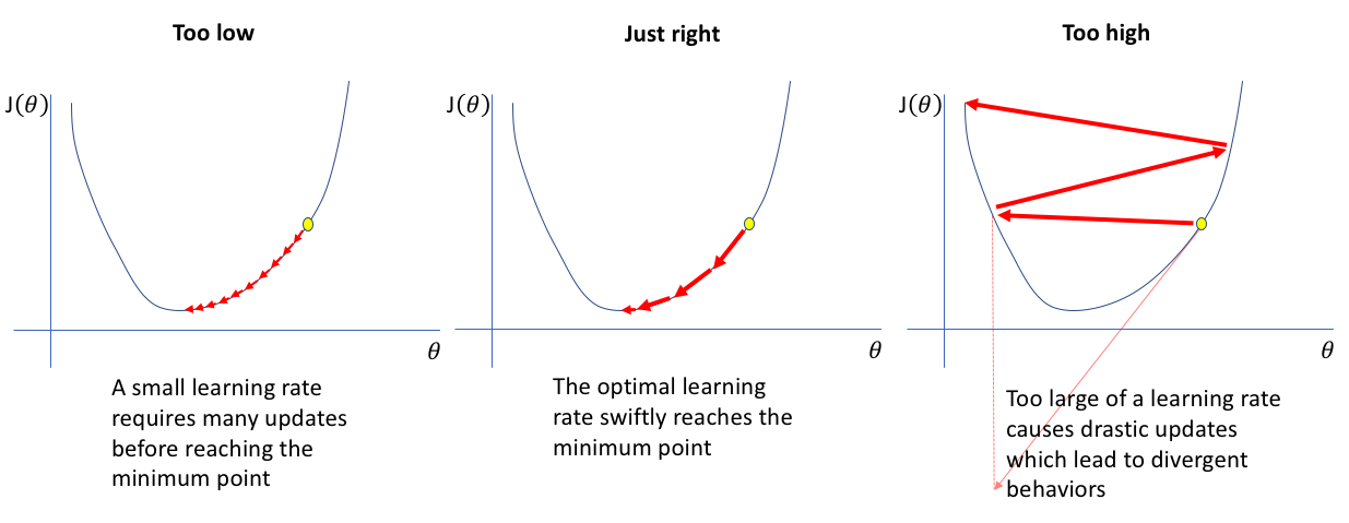
If the model learning rate is way too smaller than optimal values, it will take a much longer time (hundreds or thousands) of epochs to reach an ideal state. On the other hand, if the learning rate is much larger than optimal value, then it would overshoot the ideal state and the algorithm might not converge. A reasonable starting learning rate = 0.001.
Important to consider that: a) the model will have have hundreds and thousands of parameters each with its own error curve. And learning rate has to shepherd all of them b) error curves are not clean u-shapes; instead, they tend to have more complex shapes with local minima.
Batch size has an effect on the resource requirements of the training process, speed and number of iterations in a non-trivial way. Historically, there has been a debate to do stochastic training where you fit a single example of the dataset to the model and, using only one example, perform a forward pass, calculate the error / backpropagate & set adjusted values for all the hyperparameters. And then do this again for each example in the dataset.
Or, perhaps better to feed the entire data to the training step and calculate the gradient using the error generated by looking at all the examples in the dataset. This is called batch training.
Commonly used technique today is to set a mini-batch size. Stochastic Training is when the minibatch size =1 , and Batch Training is when the mini-batch size = Number of examples in the training set. Recommended starting values for experimentation: 1, 2, 4, 8, 16, 32, 64, 128, 256.
A larger mini-batch size allows computational boosts that utilizes matrix multiplication in the training calculations . However, it comes at expense of needing more memory for the training process. A smaller mini-batch size induces more noise in error calculations , often more useful in preventing the training process from stopping at local minima. A fair value for mini-batch size= 32.
To choose the right number of epochs for the training step, the metric we should pay attention to is the Validation Error. So, while the computational boost drives us to increase the mini-batch size, this practical algorithmic benefit incentivizes to actually make it smaller.
The intuitive manual way is to have the model train for as many number of iterations as long as validation error keeps decreasing. There’s a technique that can be used named Early Stopping to determine when to stop training the model; it is about stopping the training process in case the validation error has not improved in the past 10 or 20 epochs.
They are more involved in the structure of the model:
2.1. Number of hidden units:
Number of hidden units is one of the more mysterious hyperparameters. Let's remember that neural networks are universal function approximators, and for them to learn to approximate a function (or a prediction task) , they need to have enough ‘capacity ’ to learn the function. The number of hidden units is the main measure of model’s learning capacity.
For a simple function, it might need fewer number of hidden units. The more complex the function, the more learning capacity the model will need. Slightly more number of units then optimal number is not a problem, but a much larger number will lead to overfitting (i.e. if you provide a model with too much capacity, it might tend to overfit, trying to “memorize” the dataset, therefore affecting capacity to generalize)
2.2. First hidden layer:
Another heuristic involving the first hidden layer is that setting the number of hidden units larger than the number of inputs tends to enable better results in number of tasks, according to empirical observation.
It is often the case that 3-layer Neural Net will outperform a 2-layer one. But going even deeper rarely helps much more. (exception are Convolutional Neural Networks, where the deeper they are, the better they perform).
Hyperparameters Optimisation Techniques
The process of finding most optimal hyperparameters in machine learning is called hyperparameter optimisation.
Common algorithms include:
- Grid Search
- Random Search
- Bayesian Optimisation
Grid search is a traditional technique for implementing hyperparameters. It is somewhat about brute force all combinations. Grid search requires creatingtwo set of hyperparameters:
.Learning Rate .Number of Layers
Grid search trains the algorithm for all combinations by using the two set of hyperparameters (learning rate and number of layers) and measures the performance using cross-validation technique. This validation technique ensures the trained model gets most of the patterns from the dataset (one of the best methods to perform validation by using “K-Fold Cross Validation” which helps to provide ample data for training the model and ample data for validations).
The Grid search method is a simpler algorithm to use but it suffers if data have high dimensional space called the curse of dimensionality.

Random Search Randomly samples the search space and evaluates sets from a specified probability distribution. Instead of trying to check all 100,000 samples, for instance, we can check 1,000 random parameters.
The drawback of using the random search algorithm, however, is that it doesn’t use information from prior experiments to select the next set. Moreover, it is difficult to predict the next of experiments.
Hyperparameter setting maximizes the performance of the model on a validation set. ML algos frequently require fine-tuning of model hyperparameters. Unfortunately, that tuning is often called ‘black function’ because it cannot be written into a formula (derivatives of the function are unknown). A more appealing way to optimize & fine-tune hyperparameters entails enabling automated model tuning approach — for example, by using Bayesian optimization. The model used for approximating the objective function is called surrogate model. A popular surrogate model for Bayesian optimization is Gaussian process (GP). Bayesian optimization typically works by assuming the unknown function was sampled from a Gaussian Process (GP) and maintains a posterior distribution for this function as observations are made.
There are two major choices to be made when performing Bayesian optimization:
Select prior over functions that will express assumptions about the function being optimized. For this, we choose Gaussian Process prior; Next, we must choose an acquisition function which is used to construct a utility function from the model posterior, allowing us to determine the next point to evaluate.
A Gaussian process defines the prior distribution over functions which can be converted into a posterior over functions once we have seen some data. The Gaussian process uses Covariance matrix to ensure that values that are close together. The covariance matrix along with a mean µ function to output the expected value ƒ(x) defines a Gaussian process.
- Gaussian process will be used as a prior for Bayesian inference;
- Computing the posterior enables it to be used to make predictions for unseen test cases.
Introducing sampling data into the search space is done by acquisition functions. It helps to maximize the acquisition function to determine the next sampling point. Popular acquisition functions are .Maximum Probability of Improvement (MPI) .Expected Improvement (EI) .Upper Confidence Bound (UCB)
The Expected Improvement (EI) is a popular one and defined as:
EI(x)=𝔼[max{0,ƒ(x)−ƒ(x̂ )}]
where ƒ(x̂ ) is the current optimal set of hyperparameters. Maximising the hyperparameters will improve upon ƒ.