Test analysis on satellite images for semantic segmentation
The project is an end-to-end framework for Semantic Segmentation of Satellite Images Based on Deep Learning.
I have started by making an image analysis and later decide on a model to be built for Semantic Segmentation.
Image Segmentation can be defined as a process of classifying images at the pixel level. Each pixel of the image in output is the class to which that pixel belongs. Semantic Segmentation differs from object detection as semantic segmentation does not predict the bounding box of the object and prediction happens at the pixel level. As an output, we get a map of a location composed of 3 different categories from the multispectral satellite image.
The following versions of the libraries are used in the process of building deep neural networks
Python ==3.6.3
Opencv-contrib == 4.5.3
gdal == 3.1.4
matplotlib == 3.3.4
NumPy == 1.9.2
TensorFlow-hpu ==2.2.0
It is highly recommendable to create a new virtual environment in anaconda prompt to make sure that old dependencies installed are not altered.
- Installation can be done with pip. But it must be checked that pip is up to the date. This can be done with pip install -U pip
- Install TensorFlow 2 if it is not available in hand. Make sure to check the GPU compatibility before the installation of GPU-version. Installation can be made through pip install TensorFlow-gpu==2.2.0
- Install gdal: pip install gdal All other libraries like NumPy, matplotlib, os, glob comes as default with python
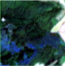
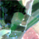
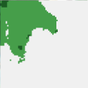
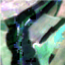
The problem is addressed with the data given composed of 5686 images and labelled into 3 different classes. Each image is from a different location specified by its geographical location. Image data is in multispectral format. It consists of 12 bands in total, while the label is a single-band image. The images are stored in .tif format. Each image is of size 64x64. Few sample images and their respective labels are shown below.


Data Directory is in format as shown below:
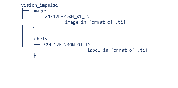
The models are to be built using 2 different types of Images. One model should make use of only Red, Blue and Green Bands. These bands are indexed at 4,3 and 2 respectively. An important point to note is Raster count starts at 1 but not at 0. The bands are extracted using a loop and the images are made by stacking the bands. Labels are simple to extract as they are of a single band. Both images and labels are segregated for training and validation
Statistics of Data :
Training Samples - 400
Validation Samples - 100
Testing Samples - 30
The limited access of GPU made usage of few samples from an entire lot of samples. Now we have data ready and the next step is to build model architecture.
There are 3 models in total which are based on Convolution Neural Networks implemented in this project:
• U_Net vanilla – Model that is trained from the base without the use of pre-trained weights
• U_Net_VGG – Model that takes the pre-trained weights of ‘imagenet’. An encoder is made of the layers extracted from the VGG framework
• DeepLab – Model that is built using ResNet50 pre-trained ‘imagenet’ weights.
Three different architectures are built and we can select one and train the model. Three models that are built are DeepLabv3, Vanilla U_Net and U_Net with the encoder of VGG pre-trained and have weights of imagenet. The model architecture is attached along with the repository.
Once the model is selected the further step is to compile the model. Adam Optimizer is used and accuracy is taken as metrics. The model is trained for 200 epochs but EarlyStopping and ModelCheckpoint are used as well to stop training if the model is not learning. Once the model is trained, predictions are made and the best weights are saved.
The model best weights are saved once the training phase of the model is done. The best weights can be used in later stages when we are willing to make predictions on new test data.
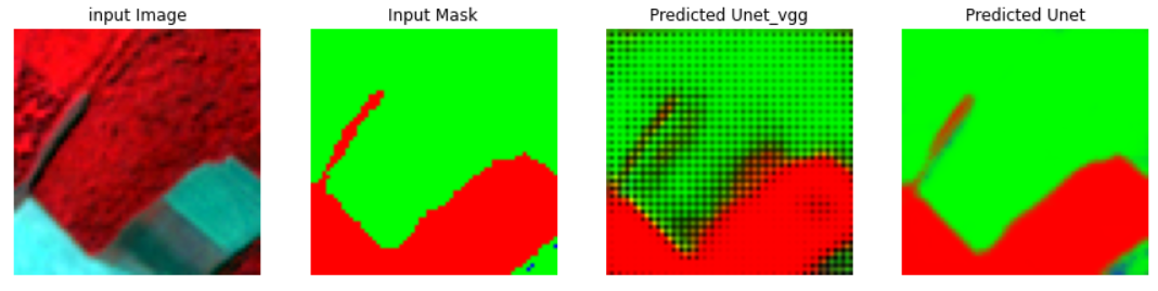
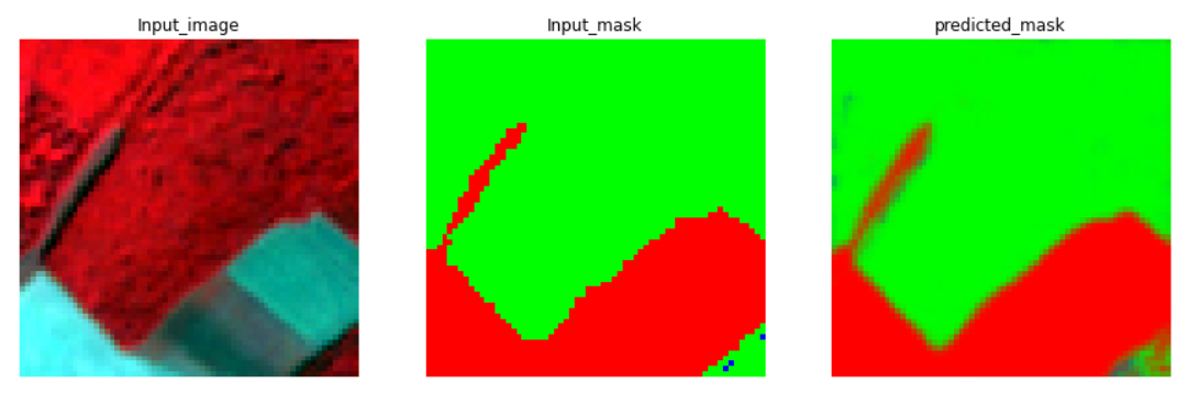
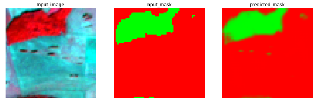
The model is then used to predict on test images. The results are given in the images.
In notebook I made a comparison of model performance by comparing the model with pre-trained weights and the model without pre-trained weights.