Surface Morphometrics Pipeline

Quantification of Membrane Surfaces Segmented from Cryo-ET or other volumetric imaging.

Author: Benjamin Barad/benjamin.barad@gmail.com, developed in close collaboration with Michaela Medina.

A pipeline of tools to generate robust open-mesh surfaces from voxel segmentations of biological membranes using the Screened Poisson algorithm, calculate morphological features including curvature and membrane–membrane distance using pycurv's vector-voting framework, and convert these morphological quantities into morphometric insights.

Everything is driven by a single morphometrics command plus a config.yml file.

📖 Complete Quantifications Documentation — reference guide for all morphological measurements and their interpretations.

Contents

• Installation
• Quick start
• Example data
• The pipeline
• Analysis & visualization
• Reference
• Troubleshooting
• Upgrading from older versions
• Dependencies
• Citation

---

Installation

Option 1: Conda (recommended)

The fastest, easiest starting point for most Linux boxes, and now for Mac as well.

1. Clone the repository: git clone https://github.com/grotjahnlab/surface_morphometrics.git
2. Create the environment (this also installs the toolkit and the morphometrics command via pip install -e .): conda env create -f environment.yml
3. Activate it: conda activate morphometrics
4. Check the install: morphometrics --help should list the pipeline subcommands.

Older Ubuntu installs (and some other Linux distributions) have known issues with graph-tool. If the main environment file fails, try conda env create -f environment-ubuntu.yml instead (tested on Ubuntu 22.04 LTS).

If you pull updates into an existing clone and the morphometrics command seems out of date, re-run pip install -e . from the repo root inside the activated environment.

Option 2: Docker

Useful on Windows and other systems where graph-tool or pymeshlab do not play nicely with conda. The image ships with all dependencies pre-installed.

git clone https://github.com/grotjahnlab/surface_morphometrics.git
cd surface_morphometrics/docker
./sm-up.sh      # build/pull, start, and enter the container
# ... run morphometrics commands inside the container ...
exit            # leave the container
./sm-down.sh    # stop the container

Start a later session the same way (cd surface_morphometrics/docker && ./sm-up.sh); end it with exit then ./sm-down.sh.

Shell completion (optional)

morphometrics is a click command, so tab-completion of subcommands and options is available. Add the matching line to your shell startup file:

# ~/.bashrc  (bash >= 4.4)
eval "$(_MORPHOMETRICS_COMPLETE=bash_source morphometrics)"
# ~/.zshrc
eval "$(_MORPHOMETRICS_COMPLETE=zsh_source morphometrics)"
# ~/.config/fish/completions/morphometrics.fish
_MORPHOMETRICS_COMPLETE=fish_source morphometrics | source

For faster shell startup, write the script to a file once (_MORPHOMETRICS_COMPLETE=zsh_source morphometrics > ~/.morphometrics-complete.zsh) and source that. (macOS ships an old bash 3.2 — use zsh, the macOS default, or install a newer bash.)

---

Quick start

Once installed, the fastest way to see the whole pipeline run is on the bundled example (a small cropped tomogram + segmentation, ~44 MB, downloaded from Zenodo):

morphometrics fetch_example          # downloads + extracts surface_morphometrics_example/
cd surface_morphometrics_example     # has tomograms/, segmentations/, and a ready config.yml

morphometrics make_meshes config.yml                 # 1. segmentations -> surface meshes
morphometrics pycurv config.yml                      # 2. curvature
morphometrics distances_orientations config.yml      # 3. distances & orientations
morphometrics sample_density config.yml              # 4. sample tomogram density (for thickness)
morphometrics measure_thickness config.yml           # 5. membrane thickness

Each command prints what to run next. See The pipeline for what every step does and how to configure it for your own data.

---

Example data

Tutorial segmentations live in example_data/:

cd example_data
tar -xzvf examples.tar.gz   # -> TE1.mrc, TF1.mrc

TE1.mrc and TF1.mrc are segmentation label volumes — enough to run the curvature and distance/orientation steps. No raw tomograms are included here (they are large), so thickness and refinement need the full-pipeline example below. You can inspect them with mrcfile:

import mrcfile
with mrcfile.open('TE1.mrc', permissive=True) as mrc:
    print(mrc.data.shape)  # (312, 928, 960)

Some MRC headers are non-standard (e.g. exported from Amira); open them with permissive=True and ignore the "file may be corrupt" warning — the toolkit still runs correctly.

Full-pipeline example (with a raw tomogram). To exercise sample_density, measure_thickness, and refine_mesh, use morphometrics fetch_example (see Quick start). The bundle is a cropped IMM+OMM sub-volume with a preconfigured config.yml (IMM=1, OMM=2). The full uncropped tomograms are on EMPIAR-12534; morphometrics fetch_example --source empiar prints how to retrieve them (hundreds of MB to GB each).

---

The pipeline

Each step reads a config.yml and writes its outputs into the configured work_dir. Steps run in order; each command prints a hint for the next one. On a 4-core laptop the tutorial datasets take a few hours end to end (the pycurv and, if used, refinement steps dominate); cluster parallelization brings this down substantially.

#	Step	Command
0	Create a config	morphometrics new_config
1	Segmentations → meshes	morphometrics make_meshes config.yml
2	Curvature (pycurv)	morphometrics pycurv config.yml
3	(optional) Mesh refinement	morphometrics refine_mesh config.yml → accept_refinement
4	Distances & orientations	morphometrics distances_orientations config.yml
5	Thickness (needs tomograms)	morphometrics sample_density config.yml → measure_thickness
6	Aggregate statistics	morphometrics stats config.yml <name>

Most steps also accept a single input (e.g. morphometrics pycurv config.yml TE1_OMM.surface.vtp, morphometrics distances_orientations config.yml TE1.mrc) so you can parallelize per tomogram on a cluster.

Configuration

morphometrics new_config writes a fully-commented config.yml into the current directory (-o NAME for a different name); edit it for your project. A few starting tips:

• For higher-quality meshes with near-equilateral triangles, set isotropic_remesh: true and simplify: false in surface_generation. target_area of 1.0–3.0 nm² works well (smaller = finer but slower).
• Set the directories and labels: seg_dir, tomo_dir, work_dir, and segmentation_values (the label value → name mapping for your segmentation).

Data organization for thickness and refinement

Thickness (step 5) and refinement (step 3) read the raw tomogram density, not just the segmentation. Three directories in config.yml control this:

• seg_dir — the segmentation MRC files (label volumes you generate surfaces from).
• tomo_dir — the raw (greyscale) tomogram MRC files the segmentations were drawn on.
• work_dir — the working/output directory where pycurv writes its graphs (.gt) and CSVs.

Each raw tomogram in tomo_dir must share the basename (the part before .mrc) of its segmentation. Tomograms are matched to surfaces by globbing work_dir for {tomogram_basename}*{component}.AVV_rh{radius_hit}.gt. For example, segmentation TE1.mrc (producing TE1_OMM.AVV_rh9.gt) needs a raw tomogram also named TE1.mrc. A typical layout:

project/
├── segmentations/   # seg_dir  ->  TE1.mrc, TF1.mrc   (label volumes)
├── tomograms/       # tomo_dir ->  TE1.mrc, TF1.mrc   (raw density, matching basenames)
└── morphometrics/   # work_dir ->  TE1_OMM.AVV_rh9.gt, ... (pycurv output + results)

A basename mismatch is the most common reason thickness or refinement "finds no files" (the tomogram is silently skipped).

Mesh refinement (optional)

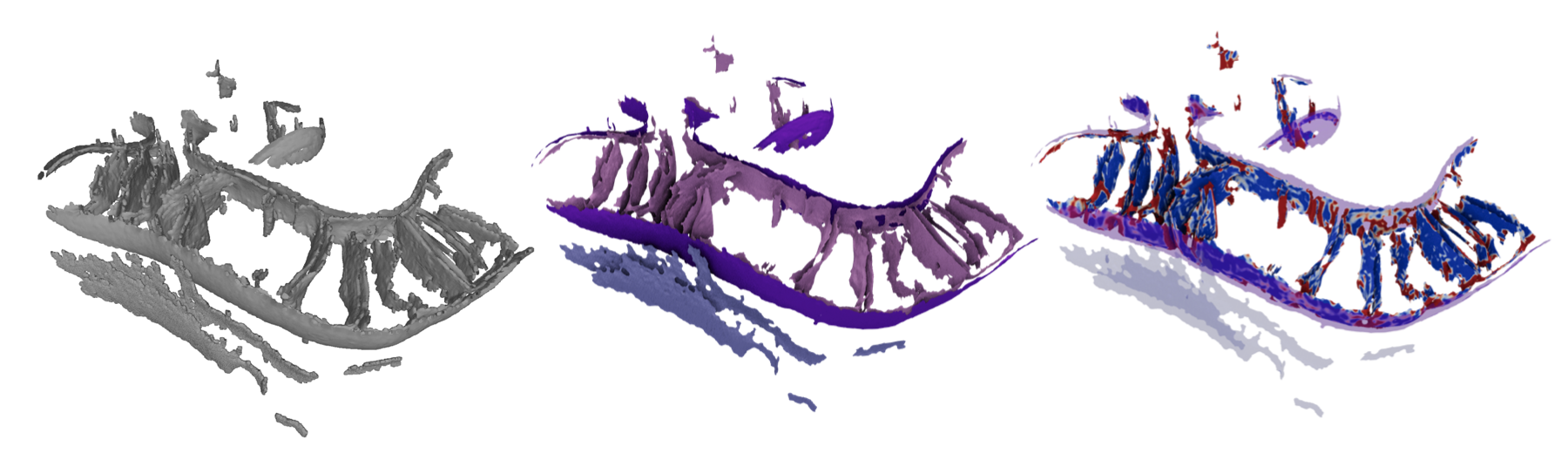
After pycurv and before the distance/thickness steps, morphometrics refine_mesh config.yml nudges surface vertices onto the true membrane bilayer center. It samples the raw tomogram density along surface normals and iteratively recenters vertices on the fitted bilayer (or, for high-defocus data, a single Gaussian), re-running pycurv each iteration. It needs raw tomograms organized as in Data organization, and is tuned via the mesh_refinement section of config.yml.

Refinement improves every surface, so it is worth running — but it is by far the slowest step (it runs pycurv internally on each Gaussian-fitting iteration, ≈ several morphometrics pycurv runs per surface). For large datasets, process one surface at a time (--tomogram/--mrc) in parallel on a cluster, or set aside time for the full run.

Refinement does not replace your working surfaces automatically. It writes a numbered surface per iteration (*_refined_iter*.surface.vtp) plus convergence plots (*_refinement_convergence.png, *_profile_evolution.png). Inspect those, then commit the best iteration:

morphometrics accept_refinement config.yml <step>      # <step> = iteration number

This backs the originals up to *.orig.bak, promotes the chosen iteration to the canonical surface (*.surface.vtp and *.AVV_rh*.gt/.vtp/.csv), and removes the other iterations and intermediates while keeping the summaries. Options: --dry-run previews all changes; --component_name OMM / --tomogram TF1 restrict to a subset.

When use_xcorr is enabled, intermediate cross-correlation iterations are saved with a fast "lightweight" graph (no curvature) — only the final iteration runs full pycurv. If you accept a lightweight iteration, the promoted surface has no *.AVV_rh*.gt graph and needs pycurv re-run first; accept_refinement warns you and prints the exact command.

---

Analysis & visualization

After the pipeline, per-triangle quantifications live in the .gt graphs, .vtp surfaces, and .csv tables in work_dir.

Statistics & plotting

The stats command (step 6) assembles an Experiment pickle across all tomograms in your data folder; from there, analysis is done in pandas (the Experiment/Tomogram classes and helpers in surface_morphometrics.morphometrics_stats). Quick single-file plots:

• morphometrics histogram filename.csv -n feature — area-weighted histogram of one feature.
• morphometrics hist2d filename.csv -n1 feature1 -n2 feature2 — area-weighted 2D histogram of two features.

Paper-specific analyses (e.g. old_scripts/mitochondria_statistics.py, which generated every plot/statistic in the preprint) live in old_scripts/ and are run directly with python from the repo root.

Protein patch and connected-component analysis (optional)

These tools tag regions of a membrane graph with an integer id so per-region statistics (curvature, thickness, etc.) can be computed and compared. They share the patch_analysis section of config.yml. Both patch and component tools write *_patches.{gt,vtp,csv} / *_components.{gt,vtp,csv}, so every per-triangle property is available for pandas.

Protein-centered patches — morphometrics generate_patches. Given a STAR file of particle coordinates (ATP synthase, ribosomes, …) and a membrane graph, places a circular patch (patch_radius nm) on the nearest membrane triangle to each particle:

morphometrics generate_patches config.yml                                    # batch over all tomograms
morphometrics generate_patches config.yml --graph TS1_IMM.AVV_rh9.gt --star TS1.star
morphometrics generate_patches config.yml --no-random                       # skip random control patches

• Each patch is identified by the particle's STAR line ID (patch_number/patch_center).
• Triangles in overlapping patches go to the nearest center; the deciding distances are stored as patch_center_distance and protein_distance.
• With generate_random: true, matched random control patches are placed (random_min_distance, reproducible via random_seed) as patch_random_number/patch_random_center, reusing ids so patch_random_number == i controls for patch_number == i.
• particle_max_distance skips particles too far from the membrane (null disables).
• Batch STAR matching: STAR files live in star_dir, matched per tomogram via star_pattern (default "{tomo}.star"); coordinate/pixel-size columns are configurable and default to RELION conventions.
• Which particles are used: by default every row in the STAR is used, so each STAR must hold only that tomogram's particles. For a combined multi-tomogram STAR, set star_tomo_column (e.g. rlnMicrographName); rows are matched to the tomogram by basename (tolerating paths, .mrc extensions, and different pixel-size/bin names like /data/TS_004.mrc_6.65Apx.mrc). patch_id stays tied to the original STAR row. Single-graph mode: --star-tomo-column/--tomo-name.
• Annotated STAR output: with annotate_star: true, writes {star}_{label}_meshannotated.star adding patch_id, mesh_distance, and mesh_neighbor_id per particle — useful for particle-side filtering (e.g. selecting cotranslating ribosomes by mesh_distance).

Connected components — morphometrics label_components. Labels each connected component with component_number (1..N by size; min_component_size drops small ones). Parallels patch_number, so the same per-region math applies:

morphometrics label_components config.yml                  # all AVV graphs
morphometrics label_components config.yml --graph TS1_IMM.AVV_rh9.gt

Per-region statistics — morphometrics patch_statistics. One property-agnostic, area-weighted aggregator for patches and components; reads the per-triangle CSVs and writes one tidy patch_statistics.csv (one row per region):

morphometrics patch_statistics config.yml                              # all *_patches.csv in work_dir
morphometrics patch_statistics config.yml --pattern "*_components.csv" # components instead
morphometrics patch_statistics config.yml --properties curvedness_VV,thickness --csv TS1_IMM.AVV_rh9_patches.csv

Auto-detects whichever label columns are present (patch_number, patch_random_number, component_number) and tags each row with region_type (patch/random/component) so real patches and controls land in one table. Reports area-weighted mean and median per property (statistics_properties), plus n_triangles and total_area. Zero/NaN values are dropped per property (--keep-zeros to keep); region id 0 is always excluded.

Arbitrary region extractor — morphometrics extract_patches. Splits a graph into independent .gt/.vtp/.csv subsets by a label column or by thresholding any vertex property:

morphometrics extract_patches config.yml --graph TS1_IMM.AVV_rh9_patches.gt --by patch_number    # one file per patch
morphometrics extract_patches config.yml --graph TS1_ER.AVV_rh9.gt --property OMM_dist --max 30   # ER within 30 nm of OMM

This workflow is ported from GrotjahnLab/patch_analysis. Still to come: the flipper-based line-scan sampling.

Exporting surfaces for Blender / visualization

morphometrics export_obj converts a quantified surface .vtp into a Wavefront OBJ + MTL with one quantification baked into the surface color — ready for Blender, MeshLab, etc.

morphometrics export_obj config.yml TS1_IMM.AVV_rh9.vtp --list-features          # see colorable arrays
morphometrics export_obj config.yml TS1_IMM.AVV_rh9.vtp --feature curvedness_VV  # one surface
morphometrics export_obj config.yml --feature thickness --cmap magma             # batch over work_dir

• Writes <base>_<feature>.obj, .mtl, and .png (the colormap image referenced via map_Kd).
• Each triangle is flat-colored by its value via per-face UVs that sample a 1D colormap strip, so per-triangle values are preserved exactly.
• Range defaults to the 2nd–98th percentile (--vmin/--vmax), any matplotlib --cmap; works on any per-triangle (or per-vertex, averaged) array.
• NaN/unmeasured triangles get a distinct swatch (--nan-color, default lightgrey; --nan-color none maps them to the low end instead).
• Output coordinates are in Angstroms by default, since downstream tools that consume the OBJ (ChimeraX, Blender molecular nodes, etc.) work in Å space. The surface's native units are read from surface_generation.angstroms and converted only as needed. Pass --scale_to_angstroms false to export in nanometres.
• Vector properties are colorable by component (e.g. --feature n_v_x, --feature OMM_dist).
• In Blender, import the OBJ (MTL/PNG are picked up automatically) and switch to Material Preview/Rendered shading.

---

Reference

Package layout and lower-level modules

The toolkit is the surface_morphometrics Python package; the pipeline steps are morphometrics subcommands, but the underlying modules can also be imported or run with python -m surface_morphometrics.<module>:

• Mesh generation (make_meshes): mrc2xyz (segmentation → point cloud), xyz2ply (screened-Poisson reconstruction + masking), ply2vtp (ply → vtp for pycurv).
• Morphology extraction: curvature (pycurv, via pycurv), refine_mesh / accept_refinement, intradistance_verticality and interdistance_orientation (wrapped by distances_orientations), sample_density + measure_thickness.
• Quantification: morphometrics_stats (pandas classes/helpers; stats assembles the Experiment pickle), plus Paraview for 3D surface mapping. See the Quantifications Documentation.

File types

• .xyz — point clouds (flat text X Y Z per line), nm or Å scale.
• .ply — surface meshes (binary), nm or Å scale; open in Meshlab and many tools.
• .surface.vtp — the same meshes in VTK format; the input pycurv reads to build graphs. Open in Paraview / pyvista.
• .AVV_rh*.vtp — pycurv outputs carrying the quantifications; richest for Paraview/pyvista visualization.
• .gt — triangle graphs (graph-tool); fast neighbor operations, not for manual inspection.
• .csv — per-triangle quantification tables; the files you use for statistics and plots.
• .log — logs, mostly from pycurv.
• Quantification outputs (plots/tests) are written as csv, svg, and png.

---

Troubleshooting

• Gaussian or Mean curvature of X has a large computation error — safe to ignore (pycurv cleans these up); they are suppressed by default.
• MRC files from AMIRA (and some other software, e.g. Dragonfly) lack proper machine stamps; open with mrcfile.open(filename, permissive=True).
• If pycurv seems to hang indefinitely, try setting cores: 1 in the config.

---

Upgrading from older versions

The toolkit is now an installable package driven by the single morphometrics command (installed by conda env create, or pip install -e . inside the env). The old python <script>.py … invocations still work for now via deprecation shims that warn and forward to the new command; they will be removed in a future release.

Two config keys were also renamed: data_dir → seg_dir, and max_triangles → simplify_max_triangles (used only when simplify: true). make_meshes warns if it detects the old names.

Old	New
python segmentation_to_meshes.py config.yml	morphometrics make_meshes config.yml
python run_pycurv.py config.yml f.surface.vtp	morphometrics pycurv config.yml f.surface.vtp
python measure_distances_orientations.py config.yml f.mrc	morphometrics distances_orientations config.yml f.mrc
python sample_density.py config.yml	morphometrics sample_density config.yml
python measure_thickness.py config.yml	morphometrics measure_thickness config.yml
python refine_mesh.py config.yml	morphometrics refine_mesh config.yml
python accept_refinement.py config.yml N	morphometrics accept_refinement config.yml N
python morphometrics_stats.py config.yml name	morphometrics stats config.yml name
python single_file_histogram.py f.csv -n feat	morphometrics histogram f.csv -n feat
python single_file_2d.py f.csv -n1 a -n2 b	morphometrics hist2d f.csv -n1 a -n2 b
(new)	morphometrics new_config — write a starter config.yml

---

Dependencies

Numpy, Scipy, Pandas, mrcfile, Click, Matplotlib, starfile, Pymeshlab, and PyCurv (which pulls in Pyto and graph-tool). The conda environment files install everything; see Installation.

---

Citation

Please cite the following if you use this toolkit (or extend it!):

Quantifying organellar ultrastructure in cryo-electron tomography using a surface morphometrics pipeline. Benjamin A. Barad^†, Michaela Medina^†, Daniel Fuentes, R. Luke Wiseman, Danielle A. Grotjahn. Journal of Cell Biology 2023, 222(4), e202204093; doi: https://doi.org/10.1083/jcb.202204093

Thickness measurement is described in:

Surface Morphometrics reveals local membrane thickness variation in organellar subcompartments. Michaela Medina^†, Ya-Ting Chang^†, Hamidreza Rahmani, Mark Frank, Zidan Khan, Daniel Fuentes, Frederick A. Heberle, M. Neal Waxham, Benjamin A. Barad^✉, Danielle A. Grotjahn^✉. Journal of Cell Biology 2025, 225(3), e202505059; doi: https://doi.org/10.1083/jcb.202505059

The toolkit relies heavily on PyCurv for vector-voted curvature and the triangle-graph framework — please also cite:

Reliable estimation of membrane curvature for cryo-electron tomography. Maria Salfer, Javier F. Collado, Wolfgang Baumeister, Rubén Fernández-Busnadiego, Antonio Martínez-Sánchez. PLOS Comp Biol August 2020; doi: https://doi.org/10.1371/journal.pcbi.1007962