RGB images have 3 channels, grayscale only 1. Number of channels appears with sci-kit as the third dimension
Some useful commands:
from skimage import data, color
rocket_image = data.rocket()
from skimage import color
grayscale = color.rgb2gray(rocket)
rgb= color.gray2rgb(grayscale)

#alternative:

from skimage.color import rgb2gray
Representing images with matplotlib:
def show_image(image, title='Image', cmap_type='gray')
plt.imshow(image, cmap=cmap_type)
plt.title(title)
plt.axis('off')
plt.show()
madrid_image= plt.imread('/madrid.jpeg')
type(madrid_image)
How to obtain colour values of an RGB image:
red= image[:, :, 0]
green= image[:, :, 1]
blue= image[:, :, 2]
The default colormap is not grayscale, we need extra coding for that:
plt.imshow(red, cmap="gray")
plt.title('Red')
plt.axis('off')
plt.show()
Shapes and dimensions:
madrid_image.shape
(426, 640, 3)
madrid_image.size
817920
# Flip the image in up direction
vertically_flipped = np.flipud(madrid_image)
show_image(vertically_flipped, 'vertically flipped image')

# Flip the image in left direction
horizontally_flipped = np.fliplr(madrid_image)
show_image(horizontally_flipped, 'horizontally flipped image')
Base for analysis, threshold, brightness/contrast and equalize.
red= image[:,:,0]
plt.hist(red.ravel(), bins= 256)
plt.title('Red Histogramn')
plt.show()
thres= 127

binary = image > thresh

show_image(image, 'original')
show_image(binary, 'thresholded')

inverted_binary = image <= thresh
show_image(image, 'original')
show_image(inverted_binary, inverted 'thresholded')
There are many ways of thresholding. Two big categories are global or histagram based, and local or adaptative (good for uneven illumination, but slower).
from skimage.filters import try_all_threshold
fig, ax = try_all_threshold(image, verbose=False)
show_plot(fig, ax)
How to calculate optimal threshold values:
# optimal global threshold
from skimage.filters import threshold_otsu
thresh = threshold_otsu(image)
binary_global = image > thresh

# optimal local threshold


from skimage.filters import threshold_local
block_size = 35
##this is local neighborhood
local_thresh = threshold_local(text_image, block_size, offset=10)
binary_local = text_image > local_thresh
- Enhancing an image
- Smoothening
- Empathize/remove features
- Sharpening
- Edge detection (e.g. Sobel method) It is a neighborhood operation
Edge detection with Sobel method:
from skimage.filters import sobel
##sobel requires a grayscale image
edge_sobel= sobel(image_coin)

def plot_comparison(original, filterd, title_filtered):
  fig, (Ax1, ax2) = plt.subplots(ncols=2, figsize=(8,6), sharex=True,
                                 sharey=True)
  ax1.imshow(original, cmap=plt.cm.gray)
  ax1.set_title('original')
  ax2.imshow(filtered, cmap=plt.cm.gray)
  ax2.set_title(title_filtered)
  ax2.axis('off')


plot_comparison(image_coin, edge_sobel, "Edge with Sobel")
Gaussian smoothing
from skimage.filters import gaussian
gaussian_image = (gaussian, original_pic, multichannel =True)
plot_comparison(original_pic, gaussian_image, "Blurred witht Gaussian filter")
Contrast enhancement (histogram equalization) Spreads out most common values
from skimage import exposure

##histogram equalization
image_eq = exposure.equalize_hist(image)
show_image(image, 'Original')
show_image(image_eq, 'Histogram equalized')

##adaptive equalization (contrastive limited adaptive histogram equalization, CLAHE)
image_adapteq = exposure.equalize_adapthist(image, clip_limit=0.03)
Medical images:
# Import the required module
from skimage import exposure

# Show original x-ray image and its histogram
show_image(chest_xray_image, 'Original x-ray')

plt.title('Histogram of image')
plt.hist(chest_xray_image.ravel(), bins=256)
plt.show()

# Use histogram equalization to improve the contrast
xray_image_eq =  exposure.equalize_hist(chest_xray_image)

# Show the resulting image
show_image(xray_image_eq, 'Resulting image')
Improve the quality of an aerial image:
from skimage import exposure
image_eq= exposure.equalize_hist(image_aerial)
show_image(image_aerial, 'Original')
show_image(image_eq, 'Resulting image')
Increase impact and contrast of an image:
from skimage import data, exposure

original_image = data.coffee()
adapthist_eq_image = exposure.equalize_adapthist(original_image, clip_limit=0.03)

show_image(original_image)
show_image(adapthist_eq_image, '#ImageprocessingDatacamp')
- Preparing images for classification ML models
- Optimization/compression
- Save images with same proportions
Rotating
from skimage.transform import rotate
image_rotated = rotate(image, -90)
show_image(image, 'original')
show_image(image_rotated, 'rotated 90 degrees anticlockwise')
##NOTE: negative values means clockwise, use positive numbers to turn left
Rescaling
##Downgrading:
from skimage.transform import rescale
image_rescaled = rescale(image, 1/4, anti-aliasing= True, multichannel=True)
Resizing is similar tu rescaling, but allows to specify dimensions
from skimage.transform import resize
##We need to give values
height = 400
width = 500
image_resized = resize(image, (height, width), anti_aliasing= True)
##this method can change the scale ratio, unless we resize proportionally:
height= image.shape[0]/4
width = image.shape[1]/4
Exercise:
# Import the module and the rotate and rescale functions
from skimage.transform import rotate, rescale

# Rotate the image 90 degrees clockwise
rotated_cat_image = rotate(image_cat, -90)

# Rescale with anti aliasing
rescaled_with_aa = rescale(rotated_cat_image, 1/4, anti_aliasing=True, multichannel=True)

# Rescale without anti aliasing
rescaled_without_aa = rescale(rotated_cat_image, 1/4, anti_aliasing=False, multichannel=True)

# Show the resulting images
show_image(rescaled_with_aa, "Transformed with anti aliasing")
show_image(rescaled_without_aa, "Transformed without anti aliasing")


# Import the module and function to enlarge images
from skimage.transform import rescale

# Import the data module
from skimage import data

# Load the image from data
rocket_image = data.rocket()

# Enlarge the image so it is 3 times bigger
enlarged_rocket_image = rescale(rocket_image, 3, anti_aliasing=True, multichannel=True)

# Show original and resulting image
show_image(rocket_image)
show_image(enlarged_rocket_image, "3 times enlarged image")


# Import the module and function
from skimage.transform import resize

# Set proportional height so its half its size
height = int(dogs_banner.shape[0] / 2)
width = int(dogs_banner.shape[1] / 2)

# Resize using the calculated proportional height and width
image_resized = resize(dogs_banner, (height, width), anti_aliasing=True)

# Show the original and resized image
show_image(dogs_banner, 'Original')
show_image(image_resized, 'Resized image')
- Filtering removes imperfections in the binary image but some also on grayscale images
- Dilation and erosion are the most used.
- The number pixels added or removed depends on the structuring element, a small image used to probe the input (in/fit, intersect/hit, or out of the object. The structuring element can have a square, diamond, cross... shape, depending.
Creating the shape (filled with 1s):
from skimage import morphology
square = morphology.square(4)
rectangle = morphology.rectangle(4,2)
Applying Erosion
from skimage import moprhology
selem=rectangle(12,6)
eroded_image=morphology.binary_erosion(image_horse, selem=selem)
plot_comparison(image_horse, eroded_image, 'Erosion')
##By default, erosion uses a cross shape unless selem is specified. It can be better or worse depending on the shape and the image.
Dilation:
from skimage import morphology
dilated_image = morphology.binary_dilation(image_horse)
plot_comparison(image_horse, dilated_image, 'Dilation')
Exercise with handwritten letters (very useful for OCR), world image
# Import the morphology module
from skimage import morphology

# Obtain the eroded shape
eroded_image_shape = morphology.binary_erosion(upper_r_image)

# See results
show_image(upper_r_image, 'Original')
show_image(eroded_image_shape, 'Eroded image')

# Import the module
from skimage import morphology

# Obtain the dilated image
dilated_image = morphology.binary_dilation(world_image)

# See results
show_image(world_image, 'Original')
show_image(dilated_image, 'Dilated image')
- Fixing damaged images. Reconstructing lost parts is called inpainting, by looking at the non-damaged regions. The damaged pixels are set as a mask
- Text removal
- Logo removal
- Object removal
from skimage.restoration import inpaint
mask = get_mask(defect_image)
restored_image=inpaint.inpaint_biharmonic(defect_image, mask, multichannel = True)
We use the function get_mask to define what is information and what is empty (black), for example:
# Initialize the mask
mask = np.zeros(image_with_logo.shape[:-1])

# Set the pixels where the logo is to 1
mask[210:290, 360:425] = 1

# Apply inpainting to remove the logo
image_logo_removed = inpaint.inpaint_biharmonic(image_with_logo,mask,multichannel=True)

# Show the original and logo removed images
show_image(image_with_logo, 'Image with logo')
show_image(image_logo_removed, 'Image with logo removed')
- Departures from the ideal signal, errors in image acquisition
We can apply noise:
# Import the module and function
from skimage.util import random_noise

# Add noise to the image
noisy_image = random_noise(fruit_image)

# Show original and resulting image
show_image(fruit_image, 'Original')
show_image(noisy_image, 'Noisy image')
And of course, most of the times, remove it using tools like total variation (TV, cartoon-like images), bilateral, wavelet or non-local
from skimage.restoration import denoise_tv_chambolle
denoised_image = denoise_tv_chambolle(noisy_image, weight=0.1, multichannel= True)
##The greater the weight, the more denoiser but also smoother image
from skimage.restoration import denoise_bilateral
denoised_image = denoise_bilateral(noisy_image, multichannel= True)
##Less smooth than TV, preserves the edges better
- Partition into segments to analyse
- The most basic system is thresholding, but there is more methods.
- Detection and isolation of elements of interest. AA superpixel is a group of pixels with similar/identical gray levels.
- Superpixels allow to get meanignful regions, computational efficiency.
- Segmentation can be supervised (e.g., we specify threshold level, as we saw earlier) or unsupervised.
- Simple linear iterative clusteric, SLIC, is unsupervised and based on superpixels
from skimage.segmentation import slic
from skimage.color import label2rgb
segments= slic(image, n_segments= 300)
##the number of segments is optional)
segmented_image = label2rgb(segments, image, kind='avg')
- Measure size
- Count number of objets
- Clasify shapes
- Requires binary images (thresholded with black background)
from skimage import measure
image= color.rgb2gray(image)
thresh = threshold_otsu(image)
thresholded_image = image > thresh

contours =measure.find_contours(thresholded_image, 0.8)
#level value between 0 and 1, the closer to 1 the more sensitive (less contours found)
show_image_contour(image, contours)
for contour in contours:
    print(contour.shape)
#This prints a (n, 2) -ndarray, with n representing the number of points making the contour
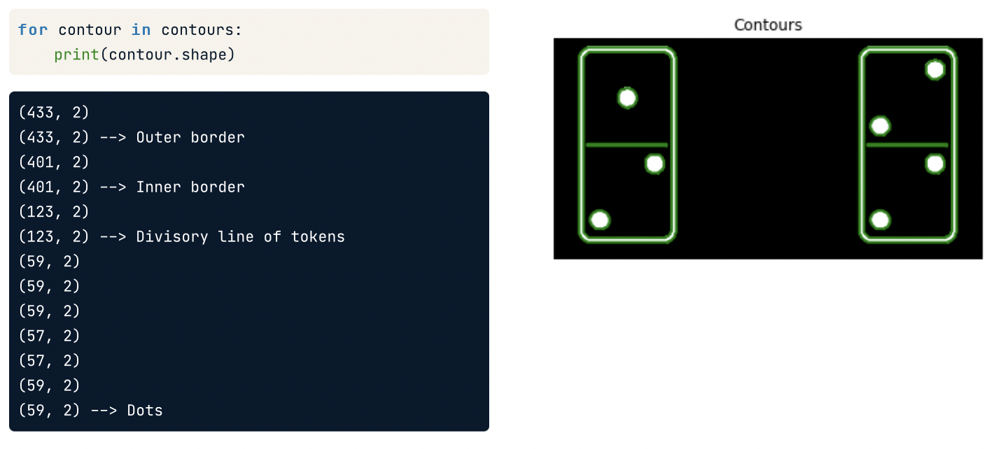
To count the number of dots in an image of dices:

# Create list with the shape of each contour
shape_contours = [cnt.shape[0] for cnt in contours]

# Set 50 as the maximum size of the dots shape
max_dots_shape = 50

# Count dots in contours excluding bigger than dots size
dots_contours = [cnt for cnt in contours if np.shape(cnt)[0] < max_dots_shape]

# Shows all contours found
show_image_contour(binary, contours)
- Using edges reduces size but retains information like shape.
- There are several filters like Sobel and Canny, considered the standard (based on gauss filtering)
- Requires grayscale image
from skimage.feature import canny
coins= color.rgb2gray(coins)
canny_edges= canny(coins)
##We can also adjust gaussian filter to remove noise. The higher, the more filter.
canny_edges_0_5 = canny(coins, sigma=0.5)
- Corner detection extracts information.
- Useful in motion detection, video tracking, 3d modeling and object recognition among others
- Points of interest are invariant to rotation, translation, intensity or scale changes. Corners and egdges are points of interest.
- A corner is the intersection of two edges, a junction of to contourns.
- We can use corner to match images on different escales, rotation, perspective...
- Harris corner detector is one of the most used methods, also requires grayscale.
from skimage.feature import corner_harris, corner_peaks
image= rgb2gray(image)
measure_image = corner_harris(image)
##Find the coordinates of the corners. The min_distance is optional
coords= corner_peaks(corner_harris(image), min_distance=5)
print("A total of", len(coords), "corners were detected.")
show_image_with_detected_corners(image, coords)
And the used function:
def show_image_with_corners(image, coords, title="Corners detected"):
plt.imshow(image, interpolation='nearest', cmap= 'gray')
plt.title(title)
plt.plot(coords[:, 1], coords[:,0], '+r', markersize=15)
plt.axis('off')
plt.show()
# Find the peaks with a min distance of 10 pixels
coords_w_min_10 = corner_peaks(measure_image, min_distance=10, threshold_rel=0.02)
print("With a min_distance set to 10, we detect a total", len(coords_w_min_10), "corners in the image.")

# Find the peaks with a min distance of 60 pixels
coords_w_min_60 = corner_peaks(measure_image, min_distance=60, threshold_rel=0.02)
print("With a min_distance set to 60, we detect a total", len(coords_w_min_60), "corners in the image.")

# Show original and resulting image with corners detected
show_image_with_corners(building_image, coords_w_min_10, "Corners detected with 10 px of min_distance")
show_image_with_corners(building_image, coords_w_min_60, "Corners detected with 60 px of min_distance")
- Used in social media, filters, auto focus, blur for privacy protection, emotion recognition and things yet to come
from skimage.feature import Cascade
##notice Cascade has cap letter!
trained_file = data.lbp_frontal_face_cascade_filename()
##data module of scikit image
detector=Cascade(trained_file)
detected= detector.detect_multi_scale(img=image, scale_Factor =1.2, step_ratio=1, min_size(10, 10), max_size(200, 200))
##scale factor deals with the search window, the higher the values, the faster but worse the search will be. The min and max windows size specify the interval for the search windows.
print(detected)
detected is a dictionary, r/c represents the position of the top left corner, then width and heigth
def show_detected_face (result, detected, title="Face image"):
plt.imshow(result)
imd_desc = plt.gca()
plt.set_cmap('gray')
plt.title(title)
plt.axis('off')

  for patch in detected:
      img_desc.add_patch(
          patches.Rectangle(
              (patch['c'], patch['r']),
              patch['width'],
              patch['height'],
              fill=False, color='r', linewidth=2)
      )

show_detected_face(image, detected)
- Measure size
- Count number of objets
- Clasify shapes
- Requires binary images (thresholded with black background)
image= color.rgb2gray(image)
- Measure size
- Count number of objets
- Clasify shapes
- Requires binary images (thresholded with black background)
image= color.rgb2gray(image)