crimerate_sf.py

# -*- coding: utf-8 -*-
"""CrimeRate_SF.ipynb

Automatically generated by Colaboratory.

Original file is located at
    https://colab.research.google.com/drive/1juxysO6SyHM7lboyeWRnWpcn7DUcwPKv

<center><h1>San Francisco Crime Classification - EDA</h1></center>

## 1. Business Problem

### 1.1. Description

Everybody has observed crimes, whether they were per- petrators or victims. Therefore, we can say- “crime is an integral part of our society”. That is why we are interested in building a crime classification system that could classify crime descriptions into different categories. A system that can help law enforcement assign the right officers to a crime or automatically assign officers to a crime based on the classification.

In our project, we analyzed the crime data that we selected from the “San Francisco Police Department (SFPD) Crime Incident Reporting System” which has the incidents of crimes in San Francisco city from 1/1/2003 to 5/13/015. So, an obvious question that can arise here is- “Why San Francisco?”

California’s San Francisco serves as the state’s administra- tive, financial, and cultural hub. It is the 17th most populous city in the US and a popular tourist destination known for its cool summers, the Golden Gate Bridge, and some of the best restaurants in the world. San Francisco is a city known for its expansion and liveliness, but because of a rise in criminal and illegal activities, it is still one of the most dangerous places to live in the US.

As per the Hoover Institution- *“San Franciscans face about a 1-in-16 chance each year of being a victim of property or violent crime, which makes the city more dangerous than 98 percent of US cities, both small and large.”* On top of that, asper an independent study by Sfgate suggests- *“San Francisco is the nearly the most crime-ridden city in the US.”* Therefore, after closely analyzing all the available data and reports we have chosen San Francisco


#### **Problem Statement**

We defined a few questions to get a sense of the security conditions in San Francisco, and we responded to them during our project- ”Crime Classification in San Francisco”.

1. How has the number of various crimes changed over time (years / months / weeks / hours / minute) in San Francisco?
2. Are there any trends in the crimes being committed over the trend?
3. Whatisthespecificlocation,time,andyearforaspecific crime?
4. Which regions are the locations where these crimes are oftenly committed?
5. Which crime (ie- theft) has highest number of occur- rences over the years in San Francisco?

### 1.2. Source/Useful Links

* Some articles and reference blogs about the problem statement.

    * https://towardsdatascience.com/deep-dive-into-sf-crime-cb8f5870a9f6
    * https://towardsdatascience.com/leveraging-geolocation-data-for-machine-learning-essential-techniques-192ce3a969bc
    * https://scottmduda.medium.com/san-francisco-crime-classification-9d5a1c4d7cfd

* Some research papers about the problem statement.

    * https://www.slideshare.net/RohitDandona/san-francisco-crime-prediction-report
    * https://www.researchgate.net/publication/305288147_San_Francisco_Crime_Classification
    * https://cseweb.ucsd.edu/classes/wi15/cse255-a/reports/fa15/012.pdf

### 1.3. Real-world/Business Objectives and Constraints

* Interpretability is important.
* Errors can be very costly.
* Probability of a data-point belonging to each class is needed.

## 2. Machine Learning Problem Formulation

### 2.1. Data Overview

* Source → https://www.kaggle.com/c/sf-crime/data
* In total, we have 3 files
    - train.csv.zip
    - test.csv.zip
    - sampleSubmission.csv.zip
    - (for time being, I have downloaded the data and unzipped it)
* The training data has 9 columns that includes target column as well.
<!--     - ![image](https://user-images.githubusercontent.com/63333753/147822986-aa8984a3-ab08-4843-9563-f242e09dcf6e.png) -->
* The test data has 6 columns that excludes target column (this is something we need to predict).
<!--     - ![image](https://user-images.githubusercontent.com/63333753/147823056-63bc4cdb-83d6-4582-8441-c9778277319f.png) -->

### 2.2. Mapping the Problem w.r.t ML Problem

#### 2.2.1. Type of ML Problem

* There are `39` different classes of the crimes that need to be classified.
* Hence this leads to multi-class classification problem.

#### 2.2.2. Performance Metric

* Source → https://www.kaggle.com/c/sf-crime/overview/evaluation
* Metric(s)
    - Multi Log-Loss
    - Confusion Matrix

#### 2.2.3. ML Objectives and Constraints

* Predict the probability of each data point belonging to each of the `39` classes.
* Constraints:
    * Interpretability
    * Class probabilities are needed.
    * Penalize the errors in class probabilites => Metric is Log-loss.
    * No latency constraints.

## 3. Exploratory Data Analysis

### 3.1. `import` Packages
"""

from google.colab import drive
drive.mount('/content/drive')

! pip install geopandas --quiet
! pip install --upgrade plotly --quiet
! pip install mpu --quiet

import warnings
warnings.filterwarnings('ignore')

import json
import os
import pickle
import pandas as pd
import numpy as np
import geopandas as gpd
import plotly.graph_objects as go
import plotly.express as px

from mpu import haversine_distance
from plotly.subplots import make_subplots
from tqdm import tqdm
from difflib import SequenceMatcher

from sklearn.preprocessing import StandardScaler
from sklearn.manifold import TSNE
from sklearn.model_selection import train_test_split
from sklearn.feature_selection import SelectKBest
from sklearn.feature_extraction.text import (
    CountVectorizer,
    TfidfVectorizer
)

from visualizer import (
    MapScatter,
    MapChoropleth,
    OccurrencePlotter,
    CategoryOccurrencePlotter
)

"""### 3.2. Data Reading

Reading `train.csv`, `test.csv`, and `sf-police-districts.shp` files
"""

project_path = '/content/drive/MyDrive/AAIC/SCS-1/sf_crime_classification/'

train_sf_df = pd.read_csv(filepath_or_buffer=project_path + 'csv_files/train.csv')
test_sf_df = pd.read_csv(filepath_or_buffer=project_path + 'csv_files/test.csv')
sf_pd = gpd.read_file(filename=project_path + 'shp_files/sf-police-districts/sf-police-districts.shp')

train_sf_df.shape, test_sf_df.shape

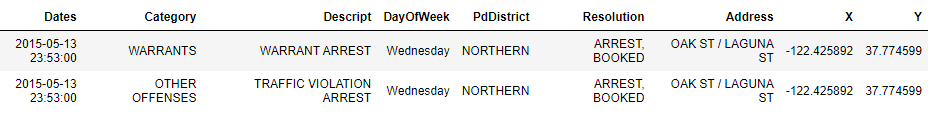
train_sf_df.head(2)

test_sf_df.head(2)

"""Renaming columns"""

train_cols_renamed = ['time', 'category', 'description', 'weekday', 'police_dept', 
                      'resolution', 'address', 'longitude', 'latitude']
train_sf_df.columns = train_cols_renamed

test_cols_renamed = ['id', 'time', 'weekday', 'police_dept', 'address', 'longitude', 'latitude']
test_sf_df.columns = test_cols_renamed

"""Removing `description` and `reolution` column from `train_sf_df`"""

train_sf_df.drop(columns=['description', 'resolution'], axis=1, inplace=True)

train_sf_df.head(2)

test_sf_df.head(2)

train_sf_df.dtypes

test_sf_df.dtypes

"""### 3.3. Time Manipulation"""

def extract_date(time):
    """Extract data from time"""
    return time.split(' ')[0]

def extract_year(date):
    """Extract year from date"""
    return int(date.split('-')[0])

def extract_month(date):
    """Extract month from date"""
    return int(date.split('-')[1])

def extract_day(date):
    """Extract day from date"""
    return int(date.split('-')[2])

def extract_hour(time):
    """Extract hour from time"""
    date, hms = time.split(' ')
    return int(hms.split(':')[0])

def extract_minute(time):
    """Extract minute from time"""
    date, hms = time.split(' ')
    return int(hms.split(':')[1])

def extract_season(month):
    """Determine season from month"""
    if month in [4, 5, 6]:
        return 'summer'
    elif month in [7, 8, 9]:
        return 'rainy'
    elif month in [10, 11, 12]:
        return 'winter'
    return 'spring'

def extract_hour_type(hour):
    """Determine hour type from hour"""
    if (hour >= 4) and (hour < 12):
        return 'morning'
    elif (hour >= 12) and (hour < 15):
        return 'noon'
    elif (hour >= 15) and (hour < 18):
        return 'evening'
    elif (hour >= 18) and (hour < 22):
        return 'night'
    return 'mid-night'

def extract_time_period(hour):
    """Determine the time period from hour"""
    if hour in [0, 1, 2, 3, 4, 5, 6, 7, 8, 9, 10, 11]:
        return 'am'
    return 'pm'

"""### 3.4. Text Titling"""

def title_text(text):
    """Title the text"""
    if isinstance(text, str):
        text = text.title()
        return text
    return text

"""### 3.5. Address Type (extraction)"""

def extract_address_type(addr):
    """Extract address type if it Street or Cross etc"""
    if ' / ' in addr:
        return 'Cross'
    addr_sep = addr.split(' ')
    addr_type = addr_sep[-1]
    return addr_type

"""### 3.6. Writing Time Based Features"""

def write_temporal_address_features(df, path):
    """Writing the temporal based features"""
    
    ### Adding temporal features
    df['date'] = df['time'].apply(func=extract_date)
    df['year'] = df['date'].apply(func=extract_year)
    df['month'] = df['date'].apply(func=extract_month)
    df['day'] = df['date'].apply(func=extract_day)
    df['hour'] = df['time'].apply(func=extract_hour)
    df['minute'] = df['time'].apply(func=extract_minute)
    df['season'] = df['month'].apply(func=extract_season)
    df['hour_type'] = df['hour'].apply(func=extract_hour_type)
    df['time_period'] = df['hour'].apply(func=extract_time_period)
    
    ### Adding address type
    df['address_type'] = df['address'].apply(func=extract_address_type)
    
    ### Text titling
    df = df.applymap(func=title_text)
    
    ### Writing
    df.to_csv(path_or_buf=path, index=None)
    
    return True

if (
    not os.path.isfile(path=project_path + 'csv_files/train_time_address_cleaned.csv') and
    not os.path.isfile(path=project_path + 'csv_files/test_time_address_cleaned.csv')
   ):
    # Training
    write_temporal_address_features(df=train_sf_df, path=project_path + 'csv_files/train_time_address_cleaned.csv')
    # Test
    write_temporal_address_features(df=test_sf_df, path=project_path + 'csv_files/test_time_address_cleaned.csv')

else:
    print("Data already exists in the directory.")
    train_sf_df = pd.read_csv(filepath_or_buffer=project_path + 'csv_files/train_time_address_cleaned.csv')
    test_sf_df = pd.read_csv(filepath_or_buffer=project_path + 'csv_files/test_time_address_cleaned.csv')

train_sf_df.head(2)

test_sf_df.head(2)

"""### 3.7. Data Description

mainly `latitude` and `longitude`
"""

train_sf_df[['latitude', 'longitude']].describe()

"""* The maximum value of the `latitude` should be around `37.7` to `38`.
* But from the above result, the max value of `latitude` is `90` which clearly indicates the wrong entry of the point.
* The same is with `longitude`.
"""

test_sf_df[['latitude', 'longitude']].describe()

"""* The maximum value of the `latitude` should be around `37.7` to `38`.
* But from the above result, the max value of `latitude` is `90` which clearly indicates the wrong entry of the point.
* The same is with `longitude`.

### 3.8. Distributions
"""

def plot_column_distribution(df, column):
    """Plot the distribution of the column from dataframe"""
    
    column_val_df = df[column].value_counts().to_frame().reset_index()
    column_val_df.columns = [column, 'count']
    
    fig = px.bar(data_frame=column_val_df, x=column, y='count')
    fig.update_layout(
        autosize=True,
        height=600,
        hovermode='closest',
        showlegend=True,
        margin=dict(l=10, r=10, t=30, b=0)
    )
    
    fig.show()
    return None

"""#### 3.8.1. Target Distribution"""

plot_column_distribution(df=train_sf_df, column='category')

"""* The above is the class distribution of the column `category`.
* Clearly we can see that `Larceny/Theft` is the most occurred type of crime in the all the years.
* The last 5 to 6 crimes are negligble, meaning they occurred very rarely.
* The data is not balanced. Therefore, while building the model it is better to do stratification based splitting.
> The above plot is based on the whole dataset.

#### 3.8.2. Address-type Distribution
"""

plot_column_distribution(df=train_sf_df, column='address_type')

"""* From the above plot, we can tell that most of the crimes occurred on `Streets` and `Crosses`.
    - `St` stands for street.
    - `Cross` signifiles the junction point.
> The above plot is based on the whole dataset.

#### 3.8.3. Police-department Distribution
"""

plot_column_distribution(df=train_sf_df, column='police_dept')

"""* `Southern` is the bay area where most of the crimes got reported.
> The above plot is based on the whole dataset.

#### 3.8.4. Year Distribution
"""

plot_column_distribution(df=train_sf_df, column='year')

"""* We know that the data is recorded from **1/1/2003** to **5/13/2015**.
    - The data of the year `2015` is not recorded fully.
* Year `2013` has more number crimes. Others also have similar occurrence range.
> The above plot is based on the whole data.

#### 3.8.5. Month Distribution
"""

plot_column_distribution(df=train_sf_df, column='month')

"""* In all of the months, we can observe that the occurrence of the crimes roughly range from `60k` to `80k`.
> The above plot is based on the whole dataset.

#### 3.8.6. Weekday (day) Distribution
"""

plot_column_distribution(df=train_sf_df, column='weekday')

"""* `Friday` is the day where most of the crimes occurred.
* `Sunday` is the day where less crimes (compared with other days) occurred.
    - This is more likely because it is a holiday.
* This distribution is almost similar.
> The above is based on the whole dataset.

#### 3.8.7. Hour Distribution
"""

plot_column_distribution(df=train_sf_df, column='hour')

"""* It is observed from the above that most of the crimes happen either in the evening or midnight.
> The above plot is based on the whole dataset.

#### 3.8.8. Minute Distribution
"""

plot_column_distribution(df=train_sf_df, column='minute')

"""* There is no direct relation between the minute and occurrrence of the crime.
* The criminal will not see the minutes from the time to proceed with his/her activity.
* Yes, the criminal will definately see if it is `00` or `30` (minutes). Hence we can notice that the minutes `00` and `30` are high.
> The above plot is based on the whole dataset.

#### 3.8.9. Season Distribution
"""

plot_column_distribution(df=train_sf_df, column='season')

"""* The distribution of all the seasons are almost similar.
* But, summer is the season where most of the crimes occurred. May be this is due to the holiday vacation.
> The above plot is based on the whole dataset.

#### 3.8.10. Time-period Distribution
"""

plot_column_distribution(df=train_sf_df, column='time_period')

"""* We can observe that most of the crimes usually happen either during the evening or at night.
> The above plot is based on the whole dataset.

#### 3.8.11. Hour-type Distribution
"""

plot_column_distribution(df=train_sf_df, column='hour_type')

"""* Morning, Mid-Night, and Night are considered to be the time period suitable for crimes to be happening.
    - Infact they have similar distribution.
* Evening and Noon are the time periods where the business usually continuous.
> The above plot is based on the whole dataset.

### 3.9. Occurrence Animations
"""

oviz = OccurrencePlotter(df=train_sf_df)

"""#### 3.9.1. Yearly

on the whole dataset
"""

oviz.plot_crime_occurrences(police_dept='Southern')

"""* The above is an animation plot showing the occurrences that had happened yearly.
* The above is the count of each occurrence type occurred in the police department.
* The most comman crime that occurred is `Larceny/Theft`.
* This is something we observed in the plot of overall occurrences in all the years.

#### 3.9.2. Monthly

in a particular year
"""

oviz.plot_crime_occurrences_by_year(year=2003, police_dept='Southern')

"""* To get the animation plot that had happened monthly, we must specify the year number.
* Even here, we observe that the crime type `Larceny/Theft` is most occurred crime.

#### 3.9.3. Daily

in a particular month
"""

oviz.plot_crime_occurrences_by_month(year=2003, month=1, police_dept='Southern')

"""* The above plot is the animation plot of the occurreces that had happened on daily basis.
* To get day wise animation, we must specify the year, and the month.
* Even here, we observe that the crime type `Larceny/Theft` or `Other-Offenses` is the most occurred crime.

#### 3.9.4. Hourly

in a particular day
"""

# oviz.plot_crime_occurrences_by_day(year=2005, month=1, day=10)

"""* The above is the animation plot of the occurrences that had happened on hourly basis.

### 3.10. Map Scatter Animations
"""

mviz = MapScatter(df=train_sf_df)

"""#### 3.10.1. Yearly

on the whole dataset
"""

mviz.map_crimes(police_dept='Richmond')

"""* The above shows the exact location of the types of crimes occurred per police department.
* This is an year wise plot and the police department that is chosen is `Richmond`.

#### 3.10.2. Monthly

in a particular year
"""

mviz.map_crimes_by_year(year=2015, police_dept='Richmond')

"""* The above is month based map plot showing all the locations of the crimes that occurred.
* The police department in the above plot is `Richmond`.

#### 3.10.3. Daily

in a particular month
"""

mviz.map_crimes_by_month(year=2003, month=2, police_dept='Richmond')

"""* The above is day based map plot showing all the locations of the crimes that occurred.
* The police department in the above plot is `Richmond`.

#### 3.10.4. Hourly

in a particular day
"""

# mviz.map_crimes_by_day(year=2003, month=2, day=6)

"""* The above is hour based map plot showing all the locations of the crimes that occurred.
* There is no police department selected, meaning it shows all the crimes.

### 3.11. Map Choropleth Animations
"""

mciz = MapChoropleth(df=train_sf_df, gdf=sf_pd)

"""#### 3.11.1. Yearly

on the whole dataset
"""

# mciz.map_crimes()

"""* The above is the choropleth map based on the count of the occurrences per police department.
* Southern is the police department where most of the crimes got reported.
* This is an year wise plot.

#### 3.11.2. Monthly

in a particular year
"""

mciz.map_crimes_by_year(year=2015)

"""* The above is the choropleth map based on the count of the occurrences per police department.
* Southern is the police department where most of the crimes got reported.
* This is a month wise plot.

#### 3.11.3. Daily

in a particular month
"""

mciz.map_crimes_by_month(year=2015, month=3)

"""* The above is the choropleth map based on the count of the occurrences per police department.
* Southern is the police department where most of the crimes got reported.
* This is a day wise plot.

#### 3.11.4. Hourly

in a particular day
"""

# mciz.map_crimes_by_day(year=2015, month=3, day=3)

"""* The above is the choropleth map based on the count of the occurrences per police department.
* This is an hour wise plot.

### 3.12. Category-wise Plots
"""

# cop = CategoryOccurrencePlotter(df=train_sf_df)

"""#### 3.12.1. Monthly (categories)"""

# cop.plot_crime_occurrences_by_month()

"""#### 3.12.2. Weekly (categories)"""

# cop.plot_crime_occurrences_by_weekday()

"""#### 3.12.3. Hourly (categories)"""

# cop.plot_crime_occurrences_by_hour()

"""### 3.13. Top `12` Crime Categories

geo-density map visualization
"""

def make_subplots_of_categories_by_year(year, df, top=12):
    """Density map subplots to show the top crimes occurred based on the year"""
    
    # San Francisco coordinates
    clat = 37.773972
    clon = -122.431297
    
    # select top 20 based on the frequency
    sf_ = df[df['year'] == year]
    category_vc = sf_['category'].value_counts().to_frame()
    categories = category_vc.index.to_list()[:top]
    
    # subplots grid
    nrows = 4; ncols = 3
    fig = make_subplots(
        rows=nrows, cols=ncols, subplot_titles=categories,
        specs=[[{"type" : "mapbox"} for i in range(ncols)] for j in range(nrows)]
    )

    r = 1; c = 1
    for name in categories:
        group = sf_[sf_['category'] == name]
        if (c > ncols):
            r += 1
            if (r > nrows): break
            c = 1
        f = go.Densitymapbox(lat=group['latitude'], lon=group['longitude'], radius=1)
        fig.add_trace(trace=f, row=r, col=c)
        c += 1
    
    fig.update_layout(
        # autosize=True,
        title=year,
        height=1000, hovermode='closest', showlegend=False,
        margin=dict(l=0, r=0, t=60, b=0)
    )

    fig.update_mapboxes(
        center=dict(lat=clat, lon=clon),
        bearing=0, pitch=0, zoom=10,
        style='carto-positron'
    )
    
    fig.show()
    return None

"""**Year** → 2003"""

# make_subplots_of_categories_by_year(year=2003, df=train_sf_df)

"""![2003_categories](https://user-images.githubusercontent.com/63333753/147853321-3420214e-7b7e-4843-b3b7-2f5be307d996.png)

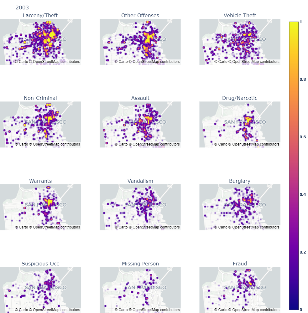
Year-wise geo-heatmap respresentation for the `top 12` crimes occurred in San Francisco

<!-- ![2003-2015_categories](https://user-images.githubusercontent.com/63333753/141100519-e53ee4fc-609f-4e07-86c9-ba9fcf2dc78f.gif) -->

#### GIF → https://bit.ly/3qFfJqM

* The GIF showcases the density map of the top 12 crimes occurred per year.
* The most important thing to observe in this is that `Larency/Theft` is always present at first.
    - The second is `Other Offenses`.
* The density is taken in descending order and hence retains the top crimes.

### 3.14. One-Hot-Encoding

Extracting time based features via OHE.
"""

def split_categories_numericals(df):
    """Identifying the numerical and categorical columns separately"""
    cols = list(df.columns)
    num_cols = list(df._get_numeric_data().columns)
    cate_cols = list(set(cols) - set(num_cols))
    return cate_cols, num_cols

ignore_columns = ['category', 'time', 'address', 'date']

def extract_feature_dummies(df, column):
    """One-Hot-Encoding using Pandas"""
    col_df = df[column]
    return pd.get_dummies(data=col_df)

def encode_multiple_columns(df, ignore_columns=ignore_columns):
    """Encoding the multiple columns and vertical stacking them"""
    cate_cols, num_cols = split_categories_numericals(df=df)
    
    multi_feature_dummies = [df[num_cols]]
    for i in cate_cols:
        if i not in ignore_columns:
            d = extract_feature_dummies(df=df, column=i)
            multi_feature_dummies.append(d)

    encoded_data = pd.concat(multi_feature_dummies, axis=1)
    
    return encoded_data

encoded_data = encode_multiple_columns(df=train_sf_df)

"""### 3.15. Extracting Spatial Distance Features"""

sf_pstations_tourists = {
    "sfpd"                : [37.7725, -122.3894],
    "ingleside"           : [37.7247, -122.4463],
    "central"             : [37.7986, -122.4101],
    "northern"            : [37.7802, -122.4324],
    "mission"             : [37.7628, -122.4220],
    "tenderloin"          : [37.7838, -122.4129],
    "taraval"             : [37.7437, -122.4815],
    "sfpd park"           : [37.7678, -122.4552],
    "bayview"             : [37.7298, -122.3977],
    "kma438 sfpd"         : [37.7725, -122.3894],
    "richmond"            : [37.7801, -122.4644],
    "police commission"   : [37.7725, -122.3894],
    "juvenile"            : [37.7632, -122.4220],
    "southern"            : [37.6556, -122.4366],
    "sfpd pistol range"   : [37.7200, -122.4996],
    "sfpd public affairs" : [37.7754, -122.4039],
    "broadmoor"           : [37.6927, -122.4748],
    #################
    "napa wine country"      : [38.2975, -122.2869],
    "sonoma wine country"    : [38.2919, -122.4580],
    "muir woods"             : [37.8970, -122.5811],
    "golden gate"            : [37.8199, -122.4783],
    "yosemite national park" : [37.865101, -119.538330],
}

def get_distance(ij):
    """Get distance from two coordinates"""
    i = ij[0]
    j = ij[1]
    distance = haversine_distance(origin=i, destination=j)
    return distance

def extract_spatial_distance_feature(df, lat_column, lon_column, pname, pcoords):
    """Compute the distance between pcoords and all the feature values"""
    lat_vals = df[lat_column].to_list()
    lon_vals = df[lon_column].to_list()
    
    df_coords = list(zip(lat_vals, lon_vals))
    pcoords_df_coords_combines = zip([pcoords] * len(df), df_coords)
    
    f = pd.DataFrame()
    distances = list(map(get_distance, pcoords_df_coords_combines))
    f[pname] = distances
    
    return f

def extract_spatial_distance_multi_features(df, lat_column, lon_column, stations=sf_pstations_tourists):
    """Compute the spatial distance for multiple features and vertical stacking them"""
    sfeatures = []
    
    for pname, pcoords in stations.items():
        print(pname, pcoords)
        sf = extract_spatial_distance_feature(df, lat_column, lon_column, pname, pcoords)
        sfeatures.append(sf)
    
    spatial_distances = pd.concat(sfeatures, axis=1)
    return spatial_distances

sd_features = extract_spatial_distance_multi_features(df=train_sf_df, lat_column='latitude', lon_column='longitude')

"""### 3.16. Extract Features only based on Latitudes and Longitudes"""

def lat_lon_sum(ll):
    """Return the sum of lat and lon"""
    lat = ll[0]
    lon = ll[1]
    return lat + lon

def lat_lon_diff(ll):
    """Return the diff of lat and lon"""
    lat = ll[0]
    lon = ll[1]
    return lon - lat

def lat_lon_sum_square(ll):
    """Return the square of sum of lat and lon"""
    lat = ll[0]
    lon = ll[1]
    return (lat + lon) ** 2

def lat_lon_diff_square(ll):
    """Return the square of diff of lat and lon"""
    lat = ll[0]
    lon = ll[1]
    return (lat - lon) ** 2

def lat_lon_sum_sqrt(ll):
    """Return the sqrt of sum of lat and lon"""
    lat = ll[0]
    lon = ll[1]
    return (lat**2 + lon**2) ** (1 / 2)

def lat_lon_diff_sqrt(ll):
    """Return the sqrt of diff of lat and lon"""
    lat = ll[0]
    lon = ll[1]
    return (lon**2 - lat**2) ** (1 / 2)

def features_by_lat_lon(df, lat_column, lon_column):
    """Compute all lat lon based features"""
    
    df_lats = df[lat_column].to_list()
    df_lons = df[lon_column].to_list()
    ll_zipped = list(zip(df_lats, df_lons))

    df_ll = pd.DataFrame()
    df_ll['lat_lon_sum'] = list(map(lat_lon_sum, ll_zipped))
    df_ll['lat_lon_diff'] = list(map(lat_lon_diff, ll_zipped))
    df_ll['lat_lon_sum_square'] = list(map(lat_lon_sum_square, ll_zipped))
    df_ll['lat_lon_diff_square'] = list(map(lat_lon_diff_square, ll_zipped))
    df_ll['lat_lon_sum_sqrt'] = list(map(lat_lon_sum_sqrt, ll_zipped))
    df_ll['lat_lon_diff_sqrt'] = list(map(lat_lon_diff_sqrt, ll_zipped))

    return df_ll

sll_features = features_by_lat_lon(df=train_sf_df, lat_column='latitude', lon_column='longitude')

"""### 3.17. BoW representation for Address"""

def create_bow_vectorizer(df, column, target='category', write_vect=True, kbest=20):
    """We should only fit on training data to avoid data leakage"""

    model_name = 'vect_bow_{}.pkl'.format(column)
    print(model_name)
    df_col_val = df[column]

    if not os.path.isfile(path=project_path + 'models/' + model_name):
        vect = CountVectorizer()
        vect.fit(raw_documents=df_col_val)
        pickle.dump(vect, open(project_path + 'models/' + model_name, "wb"))
        df_col_features = vect.transform(raw_documents=df_col_val)
    else:
        print("Model already exists in the directory.")
        vect = pickle.load(open(project_path + 'models/' + model_name, "rb"))
        df_col_features = vect.transform(raw_documents=df_col_val)

    if kbest:
        fs = SelectKBest(k=kbest)
        fs.fit(df_col_features, df[target])
        df_col_features = fs.transform(df_col_features)
    
    return pd.DataFrame(df_col_features.toarray())

train_address_bow = create_bow_vectorizer(df=train_sf_df, column='address')

"""### 3.18. TfIdf representation for Address"""

def create_tfidf_vectorizer(df, column, target='category', write_vect=True, kbest=20):
    """We should only fit on training data to avoid data leakage"""

    model_name = 'vect_tfidf_{}.pkl'.format(column)
    print(model_name)
    df_col_val = df[column]

    if not os.path.isfile(path=project_path + 'models/' + model_name):
        vect = TfidfVectorizer()
        vect.fit(raw_documents=df_col_val)
        pickle.dump(vect, open(project_path + 'models/' + model_name, "wb"))
        df_col_features = vect.transform(raw_documents=df_col_val)
    else:
        print("Model already exists in the directory.")
        vect = pickle.load(open(project_path + 'models/' + model_name, "rb"))
        df_col_features = vect.transform(raw_documents=df_col_val)

    if kbest:
        fs = SelectKBest(k=kbest)
        fs.fit(df_col_features, df[target])
        df_col_features = fs.transform(df_col_features)
    
    return pd.DataFrame(df_col_features.toarray())

train_address_tfidf = create_tfidf_vectorizer(df=train_sf_df, column='address')

"""### 3.19. Combing the data

* OHE data
* Spatial distance features
* Spatial latitude and longitude features
* Address BoW
* Address TfIdf
"""

train_sf_df_featurized = pd.concat([encoded_data, sd_features, sll_features, train_address_bow, train_address_tfidf], axis=1)
train_sf_df_featurized['category'] = train_sf_df['category']

train_sf_df_featurized.shape

"""As of now, we got 133 features.

### 3.20. Divide by Stratification
"""

def divide_by_stratification(df, target):
    """Apply stratification and split the data"""
    X = df.drop(columns=[target])
    y = df[target]
    X_train, X_test, y_train, y_test = train_test_split(X, y, test_size=0.9, stratify=y, random_state=42)
    return X_train, y_train

"""### 3.21. TSNE for Multivariate Analysis"""

def plot_tsne(X, y, k=20, perplexity=50):
    """TSNE plot after reducing the dimensionality to k best features"""
    
    fs = SelectKBest(k=k)
    fs.fit(X, y)
    X = fs.transform(X)
    print(X.shape)
    
    X = StandardScaler().fit_transform(X)
    tsne = TSNE(n_components=2, random_state=0, perplexity=perplexity)
    projections = tsne.fit_transform(X, )
    
    fig = px.scatter(projections, x=0, y=1, color=y)
    fig.update_layout(
        autosize=True,
        height=600,
        hovermode='closest',
        showlegend=True,
        margin=dict(l=10, r=10, t=30, b=0)
    )
    fig.show()

    return None

"""#### 3.21.1. Ploting TSNE for the 10% of the data

* The data is huge and we need to high have an end system to visualize TSNE for the whole data.

* For this, we are considering the all categories.
"""

X_train, y_train = divide_by_stratification(df=train_sf_df_featurized, target='category')

"""When `k = 20`"""

plot_tsne(X=X_train, y=y_train)

"""* Currently, the dataset consists of `39` classes.
* From the above plot, we can clearly see that the data is highly imbalanced.
* The clusters are not separated properly.

* **Note**: Due to in-efficiency in the system requirements, I considered only 10% of the whole data to generate the plot.

#### 3.21.2 Plottling TSNE for 10% of the data, considering the top 12 crimes

* We are neglecting all those crimes which occurred less often.
* This is just for experimentation.
"""

def segregate_only_top(df, column, n=12, randomize=True):
    """Considering only top crimes and randomizing the data"""
    top_n = df[column].value_counts().index.to_list()[:n]
    
    df_vals = []
    for i in top_n:
        df_vals.append(df[df[column] == i])
    
    df = pd.concat(df_vals, axis=0)
    if randomize:
        df = df.sample(frac=1).reset_index(drop=True)

    return df

data = segregate_only_top(df=train_sf_df_featurized, column='category')
X_train, y_train = divide_by_stratification(df=data, target='category')

"""When `k = 20`"""

plot_tsne(X=X_train, y=y_train)

"""* The above is better compared to when we considered all the categories.
* The clusters also formed in a better way.
* The separation of the clusters is also better.

#### 3.21.3. Plottling TSNE for 10% of the data, considering the top 5 crimes

* We are neglecting all those crimes which occurred less often.
* This is just for experimentation.
"""

data = segregate_only_top(df=train_sf_df_featurized, column='category', n=5)
X_train, y_train = divide_by_stratification(df=data, target='category')

"""When `k = 20`"""

plot_tsne(X=X_train, y=y_train)

"""* The above plot is far better compared to all the previous plots.
* We can see the separation clearly.
"""