| title | FEA-Driven Structural Optimization | ||||||||
|---|---|---|---|---|---|---|---|---|---|
| description | Close the loop between CadQuery geometry and FreeCAD FEM to optimize a parametric bracket through automated parameter sweeps and Pareto front analysis | ||||||||
| contributors | sam-macharia,consolata-kiiru,bright-gitari | ||||||||
| pubDate | 2026-03-04 | ||||||||
| tags |
|
||||||||
| excerpt | Build the full optimization loop: CadQuery generates parametric geometry, FreeCAD FEM meshes and solves with CalculiX, Python records results across a parameter sweep, and matplotlib visualizes the Pareto front of mass versus maximum von Mises stress. | ||||||||
| heroImage | https://cdn.siliconwit.com/education/code-based-mechanical-design/fea-driven-structural-optimization.png |
import TawkWidget from '../../../../components/TawkWidget.astro'; import UniversalContentContributors from '../../../../components/UniversalContentContributors.astro'; import InArticleAd from '../../../../components/InArticleAd.astro'; import Copyright from '../../../../components/Copyright.astro'; import BionicText from '../../../../components/BionicText.astro'; import TailwindWrapper from '../../../../components/TailwindWrapper.jsx'; import { Tabs, TabItem } from '@astrojs/starlight/components'; import { Card, CardGrid, Badge, Steps, LinkButton, FileTree } from '@astrojs/starlight/components';
import CodeBasedMechanicalDesignComments from '../../../../components/code-based-mechanical-design/CodeBasedMechanicalDesignComments.astro';
Optimizing a mechanical part by hand means changing a dimension in CAD, re-meshing in the FEA tool, running the solver, recording the result, and repeating. With three parameters and five values each, that is 125 iterations, each taking several minutes of manual work. Most engineers give up after a dozen and pick "good enough." An automated pipeline eliminates the tedium: CadQuery generates geometry, FreeCAD FEM meshes and solves with CalculiX, and Python sweeps the entire parameter space overnight. In this capstone you will build that pipeline and produce a Pareto front of mass versus stress that shows every optimal tradeoff at a glance. #FEA #StructuralOptimization #Capstone
By the end of this lesson, you will be able to:
- a parametric L-bracket in CadQuery with configurable wall thickness, rib count, fillet radius, and mounting holes
- the CadQuery-to-STEP-to-FreeCAD pipeline using Python scripting
- FreeCAD FEM analysis: mesh generation, boundary conditions, loads, and CalculiX solver settings
- a systematic parameter sweep across a 3D design space (wall thickness, rib count, fillet radius)
- results on a Pareto front to identify the optimal mass-vs-stress trade-off
The core idea is a closed-loop pipeline where geometry generation, simulation, and result extraction are all automated:
%%{init: {'flowchart': {'curve': 'linear'}}}%%
flowchart TD
    A["Parameter Set\n(thickness, ribs, fillet)"] -->|CadQuery| B["STEP\nGeometry"]
    B -->|FreeCAD API| C["Mesh +\nBCs + Loads"]
    C -->|CalculiX| D["FEA\nSolver"]
    D --> E["Extract\nMass + Stress"]
    E --> F["Store in\nData Table"]
    F -->|Next config| A
    F -->|All done| G["Pareto Front\nAnalysis"]
-
Export to STEP: CadQuery writes a STEP file that preserves exact geometry for FEM import
-
FreeCAD FEM imports and meshes: Python scripting in FreeCAD creates the FEM analysis: mesh, materials, constraints, loads
-
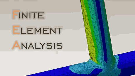
CalculiX solves: the open-source FEA solver computes displacements, stresses, and reaction forces
-
Python extracts results: read the
.frdoutput file to get maximum von Mises stress and compute mass from volume -
Record and repeat: store (parameters, mass, stress) for each configuration, then move to the next parameter combination
-
Pareto front analysis: plot mass vs. stress for all configurations and identify the non-dominated (optimal) designs
After all configurations are evaluated, matplotlib plots the Pareto front and highlights the optimal design.
The design subject is an L-bracket, a common structural element used for mounting motors, sensors, and structural connections. The bracket has:
- A horizontal base plate with mounting holes (bolted to a surface)
- A vertical web plate (carries the load)
- Optional stiffening ribs connecting the base to the web
- Fillet radii at the base-web junction (stress reduction)
import cadquery as cq
import numpy as np
from typing import Tuple

def parametric_bracket(
    base_width: float = 60.0,     # mm, base plate width (X)
    base_depth: float = 40.0,     # mm, base plate depth (Y)
    web_height: float = 50.0,     # mm, vertical web height (Z)
    wall_thickness: float = 4.0,  # mm, plate thickness
    fillet_radius: float = 4.0,   # mm, base-web junction fillet
    n_ribs: int = 2,              # number of stiffening ribs
    rib_thickness: float = None,  # mm, defaults to wall_thickness
    hole_diameter: float = 6.5,   # mm, mounting hole diameter (M6 clearance)
    hole_inset: float = 10.0,     # mm, hole center distance from edges
) -> cq.Workplane:
    """Generate a parametric L-bracket with ribs and fillets.

    The bracket sits at the origin with the base plate on the
    XY plane and the web extending upward along Z.

    Args:
        base_width: Width of the base plate (X direction)
        base_depth: Depth of the base plate (Y direction)
        web_height: Height of the vertical web (Z direction)
        wall_thickness: Thickness of plates
        fillet_radius: Fillet radius at base-web junction
        n_ribs: Number of triangular stiffening ribs
        rib_thickness: Rib thickness (defaults to wall_thickness)
        hole_diameter: Mounting hole diameter
        hole_inset: Distance from edge to hole center

    Returns:
        CadQuery solid of the bracket
    """
    t = wall_thickness
    if rib_thickness is None:
        rib_thickness = t

    # === Base plate ===
    base = (
        cq.Workplane("XY")
        .box(base_width, base_depth, t,
             centered=(True, True, False))
    )

    # === Vertical web ===
    # Web sits at the back edge of the base (Y = base_depth/2)
    web = (
        cq.Workplane("XY")
        .transformed(offset=(0, base_depth/2 - t/2, t))
        .box(base_width, t, web_height,
             centered=(True, True, False))
    )

    # Union base and web
    bracket = base.union(web)

    # === Fillet at base-web junction ===
    if fillet_radius > 0:
        # Select the interior edge where base meets web
        # Use NearestToPointSelector to target the concave junction edge
        try:
            bracket = (
                bracket
                .edges("|X")
                .edges(
                    cq.selectors.NearestToPointSelector(
                        (0, base_depth/2 - t, t)
                    )
                )
                .fillet(fillet_radius)
            )
        except Exception:
            pass  # Skip if fillet fails on complex geometry

    # === Stiffening ribs ===
    if n_ribs > 0:
        # Distribute ribs evenly across the width
        if n_ribs == 1:
            rib_positions = [0.0]
        else:
            margin = hole_inset + hole_diameter
            rib_span = base_width - 2 * margin
            rib_positions = np.linspace(
                -rib_span/2, rib_span/2, n_ribs
            ).tolist()

        rib_height = web_height * 0.7  # Ribs are 70% of web height
        rib_depth = base_depth * 0.6   # Ribs extend 60% of base depth

        for x_pos in rib_positions:
            # Triangular rib profile
            rib = (
                cq.Workplane("XY")
                .transformed(offset=(
                    x_pos, base_depth/2 - t, t
                ))
                .moveTo(0, 0)
                .lineTo(-rib_depth, 0)
                .lineTo(0, rib_height)
                .close()
                .extrude(rib_thickness)
                .translate((0, 0, 0))
            )

            # Center the rib extrusion on the x_pos
            rib = rib.translate((-rib_thickness/2, 0, 0))
            # Swap: extrude along X, so use workplane "YZ"
            rib = (
                cq.Workplane("YZ")
                .transformed(offset=(
                    x_pos - rib_thickness/2,
                    base_depth/2 - t,
                    t
                ))
                .moveTo(0, 0)
                .lineTo(-rib_depth, 0)
                .lineTo(0, rib_height)
                .close()
                .extrude(rib_thickness)
            )

            bracket = bracket.union(rib)

        # Fillet rib edges if radius permits
        if fillet_radius > 1:
            try:
                bracket = bracket.edges(
                    cq.selectors.BoxSelector(
                        (-base_width/2, -base_depth/2, t),
                        (base_width/2, base_depth/2, t + web_height)
                    )
                ).fillet(min(fillet_radius, rib_thickness * 0.4))
            except Exception:
                pass  # Skip if fillet fails on complex geometry

    # === Mounting holes in the base plate ===
    hole_positions = [
        (base_width/2 - hole_inset, base_depth/2 - hole_inset),
        (base_width/2 - hole_inset, -base_depth/2 + hole_inset),
        (-base_width/2 + hole_inset, base_depth/2 - hole_inset),
        (-base_width/2 + hole_inset, -base_depth/2 + hole_inset),
    ]

    for hx, hy in hole_positions:
        bracket = (
            bracket
            .faces("<Z")
            .workplane()
            .pushPoints([(hx, hy)])
            .hole(hole_diameter, t)
        )

    # === Load application hole in the web ===
    load_hole_z = t + web_height * 0.75  # 75% up the web
    bracket = (
        bracket
        .faces(">Y")
        .workplane()
        .pushPoints([(0, load_hole_z - t - web_height/2)])
        .hole(hole_diameter, t)
    )

    return bracket

# Generate a bracket with default parameters
bracket = parametric_bracket(
    wall_thickness=4.0,
    fillet_radius=4.0,
    n_ribs=2
)

# Export
cq.exporters.export(bracket, "bracket_t4_r2_f4.step")
import cadquery as cq
def bracket_mass(bracket: cq.Workplane,
density: float = 2.70e-6) -> float:
"""Calculate the mass of a bracket solid.
Args:
bracket: CadQuery solid
density: Material density in kg/mm³
(Aluminum 6061: 2.70e-6 kg/mm³ = 2700 kg/m³)
Returns:
Mass in grams
"""
# CadQuery volumes are in mm³
volume_mm3 = bracket.val().Volume()
mass_kg = volume_mm3 * density
mass_g = mass_kg * 1000
return mass_g
# Example
mass = bracket_mass(bracket)
print(f"Bracket volume: {bracket.val().Volume():.1f} mm³")
print(f"Bracket mass: {mass:.2f} g")import numpy as np
from itertools import product
def generate_parameter_space():
"""Define the 3D parameter sweep grid.
Returns:
List of (wall_thickness, n_ribs, fillet_radius) tuples
"""
# Wall thickness: 2.0 to 6.0 mm in 1.0 mm steps
thicknesses = [2.0, 3.0, 4.0, 5.0, 6.0]
# Rib count: 0 to 4
rib_counts = [0, 1, 2, 3, 4]
# Fillet radius: 1.0 to 8.0 mm
fillet_radii = [1.0, 2.0, 4.0, 6.0, 8.0]
# Full factorial: 5 × 5 × 5 = 125 configurations
space = list(product(thicknesses, rib_counts, fillet_radii))
print(f"Parameter space: {len(space)} configurations")
print(f" Wall thickness: {thicknesses} mm")
print(f" Rib count: {rib_counts}")
print(f" Fillet radius: {fillet_radii} mm")
return space
parameter_space = generate_parameter_space()FreeCAD's FEM workbench can be fully controlled through Python. The key objects are:
| FreeCAD Object | Purpose |
|---|---|
FemAnalysis |
Container for all FEM objects |
Fem::FemMeshGmsh |
Gmsh mesh generation |
Fem::ConstraintFixed |
Fixed boundary condition (zero displacement) |
Fem::ConstraintForce |
Applied force load |
FemMaterial |
Material properties assignment |
Fem::FemSolverCalculix |
CalculiX solver configuration |
"""
FreeCAD FEM setup script.

Run this inside FreeCAD's Python console or via:
    freecad --console script.py

This script:
1. Imports a STEP file
2. Creates a FEM analysis
3. Assigns material properties
4. Creates mesh
5. Applies boundary conditions and loads
6. Solves with CalculiX
"""
import FreeCAD
import Part
import Fem
import ObjectsFem
import Mesh
import femmesh.femmesh2mesh

def setup_fem_analysis(
    step_file: str,
    output_dir: str,
    force_magnitude: float = 500.0,  # N
    mesh_size: float = 2.0,          # mm
) -> dict:
    """Set up and run a FEM analysis on an imported STEP bracket.

    Args:
        step_file: Path to the STEP file from CadQuery
        output_dir: Directory for solver output files
        force_magnitude: Applied force in Newtons
        mesh_size: Maximum mesh element size in mm

    Returns:
        Dictionary with analysis results
    """
    # --- Create new document ---
    doc = FreeCAD.newDocument("BracketFEM")

    # --- Import STEP geometry ---
    Part.insert(step_file, doc.Name)
    shape_obj = doc.Objects[0]
    doc.recompute()

    # --- Create FEM Analysis container ---
    analysis = ObjectsFem.makeAnalysis(doc, "Analysis")

    # --- Assign material: Aluminum 6061-T6 ---
    material = ObjectsFem.makeMaterialSolid(doc, "Aluminum6061T6")
    mat_dict = material.Material
    mat_dict["Name"] = "Aluminum 6061-T6"
    mat_dict["YoungsModulus"] = "68900 MPa"
    mat_dict["PoissonRatio"] = "0.33"
    mat_dict["Density"] = "2700 kg/m^3"
    mat_dict["ThermalExpansionCoefficient"] = "23.6 µm/m/K"
    mat_dict["YieldStrength"] = "276 MPa"
    mat_dict["UltimateTensileStrength"] = "310 MPa"
    material.Material = mat_dict
    analysis.addObject(material)

    # --- Create mesh with Gmsh ---
    femmesh = ObjectsFem.makeMeshGmsh(doc, "FEMMeshGmsh")
    femmesh.Part = shape_obj
    femmesh.CharacteristicLengthMax = mesh_size
    femmesh.CharacteristicLengthMin = mesh_size / 4
    femmesh.ElementOrder = "2nd"  # Quadratic elements
    femmesh.Algorithm2D = "Frontal"
    femmesh.Algorithm3D = "Delaunay"

    # Run Gmsh meshing
    from femmesh.gmshtools import GmshTools
    gmsh = GmshTools(femmesh)
    gmsh.create_mesh()

    analysis.addObject(femmesh)
    print(f"Mesh: {femmesh.FemMesh.NodeCount} nodes, "
          f"{femmesh.FemMesh.VolumeCount} elements")

    # --- Fixed constraint on base plate bottom face ---
    fixed = ObjectsFem.makeConstraintFixed(doc, "FixedBase")
    # Select the bottom face (Z = 0)
    bottom_faces = []
    for i, face in enumerate(shape_obj.Shape.Faces):
        com = face.CenterOfMass
        if abs(com.z) < 0.1:  # Bottom face
            bottom_faces.append(
                ("Face" + str(i + 1), face)
            )

    if bottom_faces:
        fixed.References = [
            (shape_obj, bottom_faces[0][0])
        ]
    analysis.addObject(fixed)

    # --- Force load on the web hole ---
    force = ObjectsFem.makeConstraintForce(doc, "AppliedForce")
    force.Force = force_magnitude  # Newtons

    # Select the cylindrical face of the load hole
    # (the hole near the top of the web)
    load_faces = []
    for i, face in enumerate(shape_obj.Shape.Faces):
        com = face.CenterOfMass
        # Load hole is at ~75% web height, on the far Y face
        if com.z > 30 and abs(com.y) > 15:
            if face.Surface.TypeId == "Part::GeomCylinder":
                load_faces.append(("Face" + str(i + 1), face))

    if load_faces:
        force.References = [
            (shape_obj, load_faces[0][0])
        ]
    force.Direction = (shape_obj, "Face1")  # Will be corrected
    force.Reversed = False
    analysis.addObject(force)

    # --- Solver: CalculiX ---
    solver = ObjectsFem.makeSolverCalculix(doc, "CalculiX")
    solver.WorkingDir = output_dir
    solver.AnalysisType = "static"
    solver.GeometricalNonlinearity = "linear"
    solver.MaterialNonlinearity = "linear"
    solver.EigenmodesCount = 0
    solver.IterationsMaximum = 2000
    analysis.addObject(solver)

    # --- Run solver ---
    doc.recompute()

    from femtools import ccxtools
    fea = ccxtools.FemToolsCcx(analysis, solver)
    fea.update_objects()
    fea.setup_working_dir()
    fea.setup_ccx()

    message = fea.check_prerequisites()
    if message:
        print(f"Prerequisites check: {message}")
        return {"error": message}

    fea.write_inp_file()
    fea.ccx_run()
    fea.load_results()

    doc.recompute()

    return doc, analysis, solver

# Example usage (inside FreeCAD):
# doc, analysis, solver = setup_fem_analysis(
#     "bracket_t4_r2_f4.step",
#     "/tmp/bracket_fem/",
#     force_magnitude=500.0,
#     mesh_size=2.0
# )
"""
Extract results from CalculiX .frd output file.
The .frd file format contains nodal displacements, stresses,
and strains computed by CalculiX.
"""
import os
import re
import numpy as np
def extract_frd_results(frd_path: str) -> dict:
"""Parse a CalculiX .frd file to extract key results.
Args:
frd_path: Path to the .frd results file
Returns:
Dictionary with max_von_mises, max_displacement, etc.
"""
if not os.path.exists(frd_path):
raise FileNotFoundError(f"FRD file not found: {frd_path}")
von_mises_stresses = []
displacements = []
# Parse the .frd file
with open(frd_path, 'r') as f:
lines = f.readlines()
# State machine for parsing
in_stress_block = False
in_disp_block = False
for i, line in enumerate(lines):
# Detect stress results block
if "STRESS" in line and "100CL" in line:
in_stress_block = True
in_disp_block = False
continue
# Detect displacement block
if "DISP" in line and "100CL" in line:
in_disp_block = True
in_stress_block = False
continue
# End of block
if line.startswith(" -3"):
in_stress_block = False
in_disp_block = False
continue
# Parse stress data (nodal von Mises)
if in_stress_block and line.startswith(" -1"):
parts = line.split()
if len(parts) >= 7:
try:
# Columns: node, sxx, syy, szz, sxy, syz, sxz
sxx = float(parts[1])
syy = float(parts[2])
szz = float(parts[3])
sxy = float(parts[4])
syz = float(parts[5])
sxz = float(parts[6])
# Von Mises stress calculation
vm = np.sqrt(0.5 * (
(sxx - syy)**2 +
(syy - szz)**2 +
(szz - sxx)**2 +
6 * (sxy**2 + syz**2 + sxz**2)
))
von_mises_stresses.append(vm)
except (ValueError, IndexError):
continue
# Parse displacement data
if in_disp_block and line.startswith(" -1"):
parts = line.split()
if len(parts) >= 4:
try:
dx = float(parts[1])
dy = float(parts[2])
dz = float(parts[3])
disp = np.sqrt(dx**2 + dy**2 + dz**2)
displacements.append(disp)
except (ValueError, IndexError):
continue
if not von_mises_stresses:
return {"error": "No stress results found in .frd file"}
results = {
"max_von_mises_MPa": max(von_mises_stresses),
"mean_von_mises_MPa": np.mean(von_mises_stresses),
"max_displacement_mm": max(displacements) if displacements else 0,
"n_stress_nodes": len(von_mises_stresses),
"n_disp_nodes": len(displacements),
}
return results
# Alternative: Extract results from FreeCAD result object
def extract_freecad_results(doc) -> dict:
"""Extract results from FreeCAD FEM result objects.
Args:
doc: FreeCAD document with completed analysis
Returns:
Dictionary with stress and displacement results
"""
# Find the result object
result_obj = None
for obj in doc.Objects:
if hasattr(obj, "vonMises"):
result_obj = obj
break
if result_obj is None:
return {"error": "No result object found"}
von_mises = np.array(result_obj.vonMises)
disp_x = np.array(result_obj.DisplacementVectors)
# Compute displacement magnitudes
displacements = np.sqrt(
disp_x[0::3]**2 + disp_x[1::3]**2 + disp_x[2::3]**2
)
return {
"max_von_mises_MPa": float(np.max(von_mises)),
"mean_von_mises_MPa": float(np.mean(von_mises)),
"p95_von_mises_MPa": float(np.percentile(von_mises, 95)),
"max_displacement_mm": float(np.max(displacements)),
"n_nodes": len(von_mises),
}Aluminum 6061-T6 properties used throughout this analysis:
# Material: Aluminum 6061-T6
AL_6061_T6 = {
    "name": "Aluminum 6061-T6",
    "E_MPa": 68_900,           # Young's modulus
    "nu": 0.33,                # Poisson's ratio
    "rho_kg_m3": 2_700,        # Density
    "sigma_y_MPa": 276,        # Yield strength (0.2% offset)
    "sigma_ult_MPa": 310,      # Ultimate tensile strength
    "fatigue_limit_MPa": 96,   # Endurance limit at 5×10^8 cycles
    "alpha_per_C": 23.6e-6,    # Thermal expansion coefficient
}

# Design constraints for this optimization
DESIGN_CONSTRAINTS = {
    "max_von_mises_MPa": 276 / 2.0,  # σ_y / safety factor 2.0
    "max_displacement_mm": 0.5,        # Stiffness requirement
    "applied_force_N": 500,            # Load case
    "force_direction": (0, 0, -1),     # Downward (-Z)
}

print(f"Allowable stress: {DESIGN_CONSTRAINTS['max_von_mises_MPa']:.0f} MPa")
print(f"Maximum deflection: {DESIGN_CONSTRAINTS['max_displacement_mm']} mm")The driver script ties everything together: it iterates through the parameter space, generates geometry, runs FEM analysis, and collects results.
"""
Automated FEA optimization loop.

This script runs outside FreeCAD, calling it as a subprocess
for each FEM analysis. This approach is more robust than running
everything inside a single FreeCAD session (which can leak memory
over hundreds of iterations).
"""
import os
import json
import subprocess
import time
import numpy as np
from itertools import product
from typing import List, Dict, Tuple

# === Configuration ===
WORK_DIR = "/tmp/bracket_optimization/"
FREECAD_PATH = "freecadcmd"  # FreeCAD command-line executable
FORCE_N = 500.0
MESH_SIZE = 2.0  # mm

# === Parameter space ===
THICKNESSES = [2.0, 3.0, 4.0, 5.0, 6.0]
RIB_COUNTS = [0, 1, 2, 3, 4]
FILLET_RADII = [1.0, 2.0, 4.0, 6.0, 8.0]

def generate_and_export_bracket(
    t: float, n_ribs: int, r_f: float, output_dir: str
) -> Tuple[str, float]:
    """Generate a bracket and export to STEP.

    Returns:
        (step_file_path, mass_grams)
    """
    import cadquery as cq

    bracket = parametric_bracket(
        wall_thickness=t,
        fillet_radius=r_f,
        n_ribs=n_ribs,
    )

    # Calculate mass
    volume_mm3 = bracket.val().Volume()
    mass_g = volume_mm3 * 2.70e-6 * 1000  # Al 6061 density

    # Export STEP
    step_path = os.path.join(output_dir, "bracket.step")
    cq.exporters.export(bracket, step_path)

    return step_path, mass_g

def write_fem_script(
    step_path: str, output_dir: str,
    force_n: float, mesh_size: float
) -> str:
    """Write a FreeCAD Python script for FEM analysis.

    Returns the path to the generated script.
    """
    script_content = f'''
import sys
import os
import json

# Add FreeCAD paths
import FreeCAD
import Part
import Fem
import ObjectsFem

# --- Configuration ---
STEP_FILE = "{step_path}"
OUTPUT_DIR = "{output_dir}"
FORCE_N = {force_n}
MESH_SIZE = {mesh_size}
RESULTS_FILE = os.path.join(OUTPUT_DIR, "results.json")

try:
    # Create document
    doc = FreeCAD.newDocument("BracketFEM")

    # Import geometry
    Part.insert(STEP_FILE, doc.Name)
    shape = doc.Objects[0]
    doc.recompute()

    # Create analysis
    analysis = ObjectsFem.makeAnalysis(doc, "Analysis")

    # Material
    material = ObjectsFem.makeMaterialSolid(doc, "Al6061T6")
    mat = material.Material
    mat["Name"] = "Aluminum 6061-T6"
    mat["YoungsModulus"] = "68900 MPa"
    mat["PoissonRatio"] = "0.33"
    mat["Density"] = "2700 kg/m^3"
    material.Material = mat
    analysis.addObject(material)

    # Mesh
    femmesh = ObjectsFem.makeMeshGmsh(doc, "FEMMesh")
    femmesh.Part = shape
    femmesh.CharacteristicLengthMax = MESH_SIZE
    femmesh.CharacteristicLengthMin = MESH_SIZE / 4
    femmesh.ElementOrder = "2nd"

    from femmesh.gmshtools import GmshTools
    gmsh_tools = GmshTools(femmesh)
    gmsh_tools.create_mesh()
    analysis.addObject(femmesh)

    # Fixed constraint (bottom face)
    fixed = ObjectsFem.makeConstraintFixed(doc, "Fixed")
    for i, face in enumerate(shape.Shape.Faces):
        if abs(face.CenterOfMass.z) < 0.1:
            fixed.References = [(shape, "Face" + str(i+1))]
            break
    analysis.addObject(fixed)

    # Force on web hole
    force = ObjectsFem.makeConstraintForce(doc, "Force")
    force.Force = FORCE_N
    for i, face in enumerate(shape.Shape.Faces):
        com = face.CenterOfMass
        if (com.z > 30 and
            hasattr(face.Surface, 'TypeId') and
            'Cylinder' in str(face.Surface)):
            force.References = [(shape, "Face" + str(i+1))]
            break
    analysis.addObject(force)

    # Solver
    solver = ObjectsFem.makeSolverCalculix(doc, "Solver")
    solver.WorkingDir = OUTPUT_DIR
    solver.AnalysisType = "static"
    solver.GeometricalNonlinearity = "linear"
    analysis.addObject(solver)

    doc.recompute()

    # Run solver
    from femtools import ccxtools
    fea = ccxtools.FemToolsCcx(analysis, solver)
    fea.update_objects()
    fea.setup_working_dir()
    fea.setup_ccx()
    msg = fea.check_prerequisites()
    if not msg:
        fea.write_inp_file()
        fea.ccx_run()
        fea.load_results()
        doc.recompute()

        # Extract results
        import numpy as np_fc
        result_obj = None
        for obj in doc.Objects:
            if hasattr(obj, "vonMises"):
                result_obj = obj
                break

        if result_obj:
            vm = list(result_obj.vonMises)
            results = {{
                "max_von_mises_MPa": max(vm),
                "mean_von_mises_MPa": sum(vm)/len(vm),
                "n_nodes": len(vm),
                "status": "success"
            }}
        else:
            results = {{"status": "no_results"}}
    else:
        results = {{"status": "prereq_fail", "message": msg}}

except Exception as e:
    results = {{"status": "error", "message": str(e)}}

# Write results
with open(RESULTS_FILE, 'w') as f:
    json.dump(results, f, indent=2)

FreeCAD.closeDocument(doc.Name)
'''

    script_path = os.path.join(output_dir, "fem_script.py")
    with open(script_path, 'w') as f:
        f.write(script_content)

    return script_path

def run_single_analysis(
    t: float, n_ribs: int, r_f: float
) -> Dict:
    """Run one complete generate → mesh → solve cycle.

    Returns:
        Dictionary with parameters and results
    """
    # Create output directory for this configuration
    config_name = f"t{t:.0f}_r{n_ribs}_f{r_f:.0f}"
    config_dir = os.path.join(WORK_DIR, config_name)
    os.makedirs(config_dir, exist_ok=True)

    # Step 1: Generate geometry and export STEP
    step_path, mass_g = generate_and_export_bracket(
        t, n_ribs, r_f, config_dir
    )

    # Step 2: Write FEM script
    script_path = write_fem_script(
        step_path, config_dir, FORCE_N, MESH_SIZE
    )

    # Step 3: Run FreeCAD as subprocess
    try:
        result = subprocess.run(
            [FREECAD_PATH, "--console", script_path],
            capture_output=True, text=True,
            timeout=300,  # 5 minute timeout per analysis
        )
    except subprocess.TimeoutExpired:
        return {
            "t": t, "n_ribs": n_ribs, "r_f": r_f,
            "mass_g": mass_g,
            "status": "timeout"
        }

    # Step 4: Read results
    results_path = os.path.join(config_dir, "results.json")
    if os.path.exists(results_path):
        with open(results_path, 'r') as f:
            fem_results = json.load(f)
    else:
        fem_results = {"status": "no_output"}

    return {
        "t": t,
        "n_ribs": n_ribs,
        "r_f": r_f,
        "mass_g": mass_g,
        **fem_results,
    }

def run_optimization():
    """Execute the full parameter sweep."""
    os.makedirs(WORK_DIR, exist_ok=True)

    all_results = []
    total = len(THICKNESSES) * len(RIB_COUNTS) * len(FILLET_RADII)

    print(f"Starting optimization: {total} configurations")
    print("=" * 60)

    for i, (t, n_r, r_f) in enumerate(
        product(THICKNESSES, RIB_COUNTS, FILLET_RADII)
    ):
        print(f"[{i+1}/{total}] t={t}mm, ribs={n_r}, "
              f"fillet={r_f}mm ... ", end="", flush=True)

        start = time.time()
        result = run_single_analysis(t, n_r, r_f)
        elapsed = time.time() - start

        status = result.get("status", "unknown")
        if status == "success":
            sigma = result["max_von_mises_MPa"]
            print(f"OK ({elapsed:.1f}s) — "
                  f"mass={result['mass_g']:.1f}g, "
                  f"σ_max={sigma:.1f} MPa")
        else:
            print(f"FAILED ({status})")

        all_results.append(result)

    # Save all results
    output_path = os.path.join(WORK_DIR, "all_results.json")
    with open(output_path, 'w') as f:
        json.dump(all_results, f, indent=2)

    print(f"\nResults saved to: {output_path}")
    return all_results

# Run the optimization
# all_results = run_optimization()
:::tip[Practical Runtime] A 125-configuration sweep with 2mm mesh size takes approximately 2-4 hours on a modern laptop (each analysis takes 1-2 minutes). For faster iteration during development, reduce the parameter space to 3 values per dimension (27 configurations, ~30 minutes) or increase the mesh size to 3-4 mm. :::
The Pareto front identifies the non-dominated designs, configurations where no other design is simultaneously lighter AND lower stress. Any improvement in one objective requires a sacrifice in the other.
A design
-
$A$ has less mass than$B$ , AND -
$A$ has less (or equal) maximum stress than$B$
A design is Pareto-optimal if no other design in the set dominates it. The collection of all Pareto-optimal designs forms the Pareto front.
import numpy as np
from typing import List, Dict, Tuple

def find_pareto_front(
    results: List[Dict],
    obj1_key: str = "mass_g",
    obj2_key: str = "max_von_mises_MPa",
    minimize_both: bool = True,
) -> List[int]:
    """Identify Pareto-optimal designs from a set of results.

    Args:
        results: List of result dictionaries
        obj1_key: Key for objective 1 (mass)
        obj2_key: Key for objective 2 (stress)
        minimize_both: Whether both objectives should be minimized

    Returns:
        List of indices into 'results' that are Pareto-optimal
    """
    # Filter to successful results only
    valid = [
        (i, r) for i, r in enumerate(results)
        if r.get("status") == "success"
    ]

    if not valid:
        return []

    n = len(valid)
    is_dominated = [False] * n

    for i in range(n):
        if is_dominated[i]:
            continue
        idx_i, ri = valid[i]
        m_i = ri[obj1_key]
        s_i = ri[obj2_key]

        for j in range(n):
            if i == j or is_dominated[j]:
                continue
            idx_j, rj = valid[j]
            m_j = rj[obj1_key]
            s_j = rj[obj2_key]

            # Does j dominate i?
            if minimize_both:
                if m_j <= m_i and s_j <= s_i and (
                    m_j < m_i or s_j < s_i
                ):
                    is_dominated[i] = True
                    break

    pareto_indices = [
        valid[i][0] for i in range(n) if not is_dominated[i]
    ]

    return pareto_indices

def select_best_design(
    results: List[Dict],
    pareto_indices: List[int],
    max_stress_MPa: float = 138.0,  # σ_y / 2.0
    max_displacement_mm: float = 0.5,
) -> int:
    """Select the best design from the Pareto front.

    Strategy: among Pareto-optimal designs that meet all
    constraints, select the one with minimum mass.

    Args:
        results: All results
        pareto_indices: Indices of Pareto-optimal designs
        max_stress_MPa: Maximum allowable stress
        max_displacement_mm: Maximum allowable displacement

    Returns:
        Index of the best design
    """
    feasible = []
    for idx in pareto_indices:
        r = results[idx]
        if r["max_von_mises_MPa"] <= max_stress_MPa:
            feasible.append(idx)

    if not feasible:
        print("WARNING: No Pareto-optimal design meets all "
              "constraints. Returning lowest-stress design.")
        return min(pareto_indices,
                   key=lambda i: results[i]["max_von_mises_MPa"])

    # Among feasible Pareto designs, pick lightest
    best = min(feasible, key=lambda i: results[i]["mass_g"])
    return best
import matplotlib.pyplot as plt
import matplotlib.patches as mpatches
import numpy as np
def plot_pareto_front(
results: List[Dict],
pareto_indices: List[int],
best_index: int = None,
constraint_stress: float = 138.0,
title: str = "Bracket Optimization: Mass vs. Max Stress"
):
"""Plot the Pareto front with all design points.
Args:
results: All result dictionaries
pareto_indices: Indices of Pareto-optimal designs
best_index: Index of the selected best design
constraint_stress: Maximum allowable stress line
"""
fig, ax = plt.subplots(1, 1, figsize=(10, 7))
# Separate valid results
valid = [
(i, r) for i, r in enumerate(results)
if r.get("status") == "success"
]
masses = [r["mass_g"] for _, r in valid]
stresses = [r["max_von_mises_MPa"] for _, r in valid]
indices = [i for i, _ in valid]
# Color by rib count for insight
rib_counts = [r["n_ribs"] for _, r in valid]
scatter = ax.scatter(
masses, stresses,
c=rib_counts, cmap='viridis',
s=40, alpha=0.5, edgecolors='gray',
linewidth=0.5, zorder=2
)
cbar = plt.colorbar(scatter, ax=ax, label='Rib Count')
# Highlight Pareto front
pareto_masses = [results[i]["mass_g"] for i in pareto_indices]
pareto_stresses = [
results[i]["max_von_mises_MPa"] for i in pareto_indices
]
# Sort Pareto points by mass for a clean line
pareto_sorted = sorted(
zip(pareto_masses, pareto_stresses)
)
pm_sorted = [p[0] for p in pareto_sorted]
ps_sorted = [p[1] for p in pareto_sorted]
ax.plot(pm_sorted, ps_sorted, 'r-o',
markersize=8, linewidth=2,
label='Pareto front', zorder=3)
# Highlight best design
if best_index is not None:
bm = results[best_index]["mass_g"]
bs = results[best_index]["max_von_mises_MPa"]
ax.plot(bm, bs, 'r*', markersize=20, zorder=5)
ax.annotate(
f'BEST DESIGN\n'
f't={results[best_index]["t"]}mm, '
f'ribs={results[best_index]["n_ribs"]}, '
f'fillet={results[best_index]["r_f"]}mm\n'
f'mass={bm:.1f}g, σ={bs:.0f} MPa',
xy=(bm, bs),
xytext=(bm + 5, bs + 20),
fontsize=9,
arrowprops=dict(arrowstyle='->', color='red',
linewidth=2),
bbox=dict(boxstyle='round,pad=0.4',
facecolor='lightyellow',
edgecolor='red', alpha=0.9),
zorder=6
)
# Constraint line
ax.axhline(y=constraint_stress, color='orange',
linestyle='--', linewidth=1.5,
label=f'Stress limit ({constraint_stress} MPa)')
# Feasible region shading
ax.axhspan(0, constraint_stress, alpha=0.05,
color='green', label='Feasible region')
# Labels and formatting
ax.set_xlabel('Mass (g)', fontsize=13)
ax.set_ylabel('Max von Mises Stress (MPa)', fontsize=13)
ax.set_title(title, fontsize=14, fontweight='bold')
ax.legend(loc='upper right', fontsize=10)
ax.grid(True, alpha=0.3)
# Add design direction arrows
ax.annotate('', xy=(min(masses)*0.95, min(stresses)*0.9),
xytext=(max(masses)*0.5, max(stresses)*0.5),
arrowprops=dict(arrowstyle='->',
color='green', linewidth=2))
ax.text(min(masses)*1.05, min(stresses)*0.95,
'Ideal\ndirection',
fontsize=9, color='green', style='italic')
plt.tight_layout()
plt.savefig("pareto_front.png", dpi=150, bbox_inches='tight')
plt.show()
return fig
# Usage:
# pareto_idx = find_pareto_front(all_results)
# best_idx = select_best_design(all_results, pareto_idx)
# plot_pareto_front(all_results, pareto_idx, best_idx)import pandas as pd
def results_summary_table(
results: List[Dict],
pareto_indices: List[int],
best_index: int
) -> pd.DataFrame:
"""Create a summary table of all valid results.
Highlights Pareto-optimal and best designs.
"""
rows = []
for i, r in enumerate(results):
if r.get("status") != "success":
continue
rows.append({
"Config #": i,
"t (mm)": r["t"],
"Ribs": r["n_ribs"],
"Fillet (mm)": r["r_f"],
"Mass (g)": round(r["mass_g"], 1),
"σ_max (MPa)": round(r["max_von_mises_MPa"], 1),
"Pareto?": "Yes" if i in pareto_indices else "",
"Best?": ">>> BEST <<<" if i == best_index else "",
})
df = pd.DataFrame(rows)
# Sort by mass
df = df.sort_values("Mass (g)").reset_index(drop=True)
return df
# Usage:
# df = results_summary_table(all_results, pareto_idx, best_idx)
# print(df.to_string())
# df.to_csv("optimization_results.csv", index=False)The Pareto front reveals fundamental engineering trade-offs:
1. **Light designs with high stress** (left side of the Pareto front): thin walls, no ribs, small fillets. These are mass-optimal but may not meet strength requirements.-
Heavy designs with low stress (right side of the Pareto front): thick walls, many ribs, large fillets. These are over-designed and wasteful.
-
The "knee" of the Pareto front: the region of diminishing returns where adding more mass yields progressively less stress reduction. The best designs are often near this knee.
-
Infeasible designs: configurations above the stress constraint line fail the strength requirement regardless of mass. These are eliminated from consideration.
-
Dominated designs: configurations that are neither on the Pareto front nor infeasible. Another design exists that is both lighter and stronger.
The parameter sweep also reveals which design variables have the strongest influence:
import matplotlib.pyplot as plt
import numpy as np

def sensitivity_analysis(results: List[Dict]):
    """Analyze how each parameter affects mass and stress.

    Creates box plots showing the distribution of stress
    for each value of each design parameter.
    """
    valid = [r for r in results if r.get("status") == "success"]

    fig, axes = plt.subplots(2, 3, figsize=(14, 8))

    params = [
        ("t", "Wall Thickness (mm)", [2, 3, 4, 5, 6]),
        ("n_ribs", "Rib Count", [0, 1, 2, 3, 4]),
        ("r_f", "Fillet Radius (mm)", [1, 2, 4, 6, 8]),
    ]

    for col, (key, label, values) in enumerate(params):
        # Stress sensitivity
        stress_data = []
        for v in values:
            stresses = [
                r["max_von_mises_MPa"] for r in valid
                if r[key] == v
            ]
            stress_data.append(stresses)

        axes[0, col].boxplot(stress_data, labels=values)
        axes[0, col].set_xlabel(label)
        axes[0, col].set_ylabel("Max σ_vM (MPa)")
        axes[0, col].set_title(f"Stress vs. {label}")
        axes[0, col].grid(True, alpha=0.3)

        # Mass sensitivity
        mass_data = []
        for v in values:
            masses = [
                r["mass_g"] for r in valid
                if r[key] == v
            ]
            mass_data.append(masses)

        axes[1, col].boxplot(mass_data, labels=values)
        axes[1, col].set_xlabel(label)
        axes[1, col].set_ylabel("Mass (g)")
        axes[1, col].set_title(f"Mass vs. {label}")
        axes[1, col].grid(True, alpha=0.3)

    plt.suptitle("Parameter Sensitivity Analysis", fontsize=14,
                 fontweight='bold')
    plt.tight_layout()
    plt.savefig("sensitivity_analysis.png", dpi=150)
    plt.show()

# sensitivity_analysis(all_results)
Typical findings for the L-bracket problem:
| Parameter | Effect on Stress | Effect on Mass | Sensitivity |
|---|---|---|---|
| Wall thickness |
Strong reduction (inverse square) | Strong increase (linear) | Highest |
| Rib count |
Moderate reduction (ribs brace the junction) | Small increase per rib | Medium |
| Fillet radius |
Moderate reduction (stress concentration relief) | Negligible increase | Medium (stress only) |
:::note[Key Insight] Wall thickness dominates both objectives, making it the primary design lever. Fillet radius is almost "free" because it reduces stress with negligible mass penalty. Ribs provide moderate stress reduction at moderate mass cost. The optimal strategy is usually: maximize fillet radius first, add 1-2 ribs, then find the minimum wall thickness that meets the stress constraint. :::
Here is the end-to-end sequence you would run to complete this capstone project:
1. **Set up the environment** ```bash pip install cadquery numpy scipy matplotlib pandas # Ensure FreeCAD is installed with FEM workbench # Ensure CalculiX (ccx) is on the system PATH which ccx # Should return the CalculiX solver path ```-
Define the parametric bracket in CadQuery (code above) and test with a single configuration
-
Verify FEM setup by running a single analysis manually in FreeCAD to confirm mesh quality, boundary conditions, and load application are correct
-
Run the parameter sweep: start with a coarse grid (3 values per parameter = 27 configurations) to verify the pipeline, then expand to the full grid (125 configurations)
-
Compute the Pareto front and generate the visualization
-
Select the optimal design from the Pareto front and regenerate the final bracket in CadQuery
-
Final verification: run one last FEM analysis at finer mesh size (1mm) to confirm the stress result converges
-
Export production files: STEP for CNC machining, STL for 3D printing
def export_final_design(
    results: List[Dict],
    best_index: int,
    output_dir: str = "./final_bracket/"
):
    """Generate and export the final optimized bracket.

    Creates STEP, STL, and a design report.
    """
    import cadquery as cq
    import json
    import os

    os.makedirs(output_dir, exist_ok=True)
    r = results[best_index]

    # Regenerate the optimal bracket
    bracket = parametric_bracket(
        wall_thickness=r["t"],
        fillet_radius=r["r_f"],
        n_ribs=r["n_ribs"],
    )

    # Export geometry
    step_path = os.path.join(output_dir, "bracket_optimized.step")
    stl_path = os.path.join(output_dir, "bracket_optimized.stl")
    cq.exporters.export(bracket, step_path)
    cq.exporters.export(bracket, stl_path)

    # Design report
    report = {
        "project": "L-Bracket Structural Optimization",
        "material": "Aluminum 6061-T6",
        "design_parameters": {
            "wall_thickness_mm": r["t"],
            "rib_count": r["n_ribs"],
            "fillet_radius_mm": r["r_f"],
        },
        "performance": {
            "mass_g": round(r["mass_g"], 2),
            "max_von_mises_stress_MPa": round(
                r["max_von_mises_MPa"], 1
            ),
            "allowable_stress_MPa": 138.0,
            "safety_factor": round(
                138.0 / r["max_von_mises_MPa"], 2
            ),
        },
        "load_case": {
            "applied_force_N": 500,
            "direction": "Downward (-Z) on web hole",
            "boundary_condition": "Fixed base plate (4 bolt holes)",
        },
        "optimization": {
            "total_configurations_evaluated": len(results),
            "pareto_optimal_count": len([
                i for i in range(len(results))
                if i in find_pareto_front(results)
            ]),
            "solver": "CalculiX",
            "mesh_type": "2nd order tetrahedral",
        },
        "files": {
            "step": os.path.basename(step_path),
            "stl": os.path.basename(stl_path),
        }
    }

    report_path = os.path.join(output_dir, "design_report.json")
    with open(report_path, 'w') as f:
        json.dump(report, f, indent=2)

    print(f"\n{'='*50}")
    print(f"FINAL OPTIMIZED BRACKET")
    print(f"{'='*50}")
    print(f"Wall thickness:  {r['t']} mm")
    print(f"Rib count:       {r['n_ribs']}")
    print(f"Fillet radius:   {r['r_f']} mm")
    print(f"Mass:            {r['mass_g']:.1f} g")
    print(f"Max stress:      {r['max_von_mises_MPa']:.1f} MPa")
    print(f"Safety factor:   "
          f"{138.0 / r['max_von_mises_MPa']:.2f}")
    print(f"{'='*50}")
    print(f"STEP: {step_path}")
    print(f"STL:  {stl_path}")
    print(f"Report: {report_path}")

    return bracket

# Export the final design
# final_bracket = export_final_design(all_results, best_idx)This capstone brings together every technique from the course:
**Standards-driven parametric design.** You built reusable functions that generate geometry from lookup tables and equations, the same pattern used for the bracket's parametric dimensions. **Mathematical curve generation.** The involute tooth profile, contact ratio, and Lewis stress equations demonstrated how engineering math becomes CadQuery geometry, the same approach used for helix generation in springs and implicit surfaces in lattices. **Data-driven geometry.** Parsing external data (KiCad PCB files) to auto-generate geometry taught the pattern of reading inputs and producing parametric output, the same pattern the optimization loop uses when reading FEA results. **Parameter sweeps and visualization.** Sweeping fin count, height, and spacing while plotting thermal resistance maps established the optimization workflow that this capstone extends to full FEA-in-the-loop. **Advanced geometry generation.** TPMS implicit surfaces and voxel-based modeling showed that CadQuery + NumPy can handle geometry far beyond traditional CAD, the same computational approach that makes large parameter sweeps feasible. **Stress verification.** Wahl correction, Goodman fatigue analysis, and material selection from standards demonstrated rigorous engineering verification, the same mindset applied to FEA-based stress checking in this capstone. The manual version of this workflow (model a bracket in GUI CAD, import to FEM, set up analysis, run, record stress, repeat 125 times) would take weeks. The automated version runs overnight. Real engineering rarely has one "best" answer. The Pareto front shows the full trade-off landscape, letting you make informed decisions based on which constraint matters most for your application. Every aspect of this optimization (geometry, loads, constraints, solver settings, post-processing) is captured in version-controlled Python scripts. Anyone can reproduce, verify, and extend the results. Always verify the FEM setup manually on one configuration before automating. A bug in the load application that runs silently through 125 configurations wastes hours and produces meaningless results.:::tip[Next Steps] This capstone used a structured parameter sweep (full factorial grid). For higher-dimensional problems (5+ design variables), a full factorial grid becomes computationally prohibitive. Consider these advanced approaches:
- Latin Hypercube Sampling: efficiently sample high-dimensional spaces
- Bayesian Optimization (e.g., with
scikit-optimize): surrogate model guides the search to promising regions - Genetic Algorithms (e.g., with
pymoo): evolve a population of designs toward the Pareto front - Topology Optimization: let the solver decide where to place material, then interpret the result as a parametric design
These techniques build naturally on the automated pipeline you implemented here. :::