import numpy as np
import matplotlib
import matplotlib.pyplot as plt
from matplotlib.patches import Rectangle
import time
# (1) Defines a function f(x,y) for 0≤x≤1 and 0≤y≤1 .
def funxy(choice):
if choice.lower() == "random":
x = np.random.uniform(0,1,1)[0]
y = np.random.uniform(0,1,1)[0]
else:
answer = choice.split(",")
x1 = float(answer[0].strip())
y1 = float(answer[1].strip())
while x1 > 1:
x1 = x1 / 10
while y1 > 1:
y1 = y1 / 10
x = x1
y = y1
return x,y
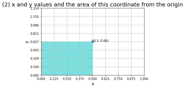
# (2) Method 1. Using the general python programming approach (Workshop sections 1 to 5), write a piece of code that calculates
# the area, A1 , inside the square 0≤x,y≤1 within which f(x,y)>0 . To do this, create a grid of x and y values with
# number of points N>1 , and use 'for' or 'while' loops to calculate the area. Your code should be general to work with
# any function f(x,y) .
choice = input("(1) Please enter x and y values by putting comma between them (x,y) or type 'random' for random x and y values:\n")
x,y = funxy(choice) # Retrieving random x and y values
print("\n\n\n")
print("x and y values which are going to be used for question 2 and 3.\n")
print("x:",x,"y:",y)
print("\n\n\n")
# Creating a graph of x and y values and shows the area
plt.figure()
currentAxis = plt.gca()
currentAxis.add_patch(Rectangle((0, 0), x, y, color = 'C', alpha=0.5))
plt.title("(2) x and y values and the area of this coordinate from the origin", fontsize=18)
plt.text(x, y, (round(x,2),round(y,2)), fontdict=None, withdash=False)
plt.xlim(0,x*2)
plt.ylim(0,y*2)
plt.xticks(np.linspace(0,x*2,9))
plt.yticks(np.linspace(0,y*2,9))
plt.xlabel("x",fontsize=14)
plt.ylabel("y",fontsize=14)
plt.grid()
plt.scatter(x,y,s=50,color="C0")
plt.show()
print("\n\n\n")
# Timer starts
start_time_all = time.perf_counter()
# Creating arrays of x and y
xRange = []
xZeros = []
yRange = []
yZeros = []
# Number of points
stepNumber = 50
# Step Sizes
xSteps = x / stepNumber
ySteps = y / stepNumber
xSum = 0
ySum = 0
# Filling the values of x and y arrays
for i in range(stepNumber+1):
xRange.append(xSum)
xZeros.append(y)
yRange.append(ySum)
yZeros.append(x)
xSum = round(xSum,4) + xSteps
ySum = round(ySum,4) + ySteps
# Reversing Arrays for plotting
xRangeRev = xRange[::-1]
yRangeRev = yRange[::-1]
# X,Y Grid Figure
plt.figure()
plt.scatter(xRangeRev,xZeros)
plt.scatter(yZeros,yRangeRev)
plt.title("(2) METHOD 1 (FOR LOOP) \n x and y values and a grid showing the area under the coordinate", fontsize=18)
plt.text(x, y, (round(x,2),round(y,2)), fontdict=None, withdash=False)
plt.xlim(0,x*2)
plt.ylim(0,y*2)
plt.xticks(np.linspace(0,x*2,9))
plt.yticks(np.linspace(0,y*2,9))
plt.xlabel("x",fontsize=14)
plt.ylabel("y",fontsize=14)
plt.grid()
plt.show()
# Calculating the area
# Due to I was a bit confused about the correct solution, I added a couple of different solutions for this question
# But the last one is used for the calculation of execution time.
# SOLUTION 1
# Considering there is a grid and this grid contains many little rectangles inside it,
# if we multiply the edges of each little rectangle and sum them up,
# we obtain the area of the big rectangle.
#xSum = 0
#ySum = 0
#for j in range(stepNumber):
# for k in range(stepNumber-1):
# ySum = ySum + round(xSteps*ySteps,2)
# xSum = xSum + ySum
#area = round(xSum,2)
# SOLUTION 2
# Instead of calculating the are of each little rectangle and summing them up,
# we may consider this grid as a matrix and moved along the each axis of the matrix
# till we reach the coordinate point. During this calculation, for loop has been
# used. (This calculation is much more efficient than the previous one. Because
# it does not calculate anything till reaching the correct coordinates.)
# for j in range(0,stepNumber):
# for k in range(0,stepNumber):
# if (xRange[j], yRange[k]) == (x, y):
# area = xRange[j]*yRange[k]
# break
# k = k + 1
# j = j + 1
# area = round(xRange[j]*yRange[k],2)
# SOLUTION 3
# As another option, we can use a dictionary as below. Keys are the coordinates
# of the matrix and the values are the multiplication of the specified coordinates.
# Basically, the last element of the dictionary gives us the area.
# This solution is not that efficient as "Solution 1" or Solution 2". Because this
# method creates matrixes everytime it runs.
start_time = time.perf_counter()
grid = {}
for row in range(len(xRange)):
for column in range(len(yRange)):
grid[row,column] = round(xRange[row]*yRange[column],2)
area = grid.get((len(xRange)-1,len(yRange)-1))
# Timers stops
Execution_time = time.perf_counter() - start_time
Execution_time_all = time.perf_counter() - start_time
print("(2) Calculated Area: {} unit".format(area))
print("(4) For Loop Execution Time including plotting graph: {} ms (milliseconds)".format(round(Execution_time_all*1000,2)))
print("(4) For Loop Execution Time excluding plotting graph: {} ms (milliseconds)".format(round(Execution_time*1000,2)))
print("\n\n\n")
# (3) Method 2. Now write another piece of code that uses Numpy for the same task. Do not use for or while loops in this case.
# Hint: work with a N×N matrix representing your (x,y) coordinate grid.
# Timer starts
start_time_all = time.perf_counter()
# Number of points
stepNumber = 50
# Filling the X and Y arrays
xRange = np.linspace(0,x,stepNumber)
yRange = np.linspace(0,y,stepNumber)
xZeros = np.repeat(y,len(xRange))
yZeros = np.repeat(x,len(yRange))
# Reversing Arrays for plotting
xRangeRev = xRange[::-1]
yRangeRev = yRange[::-1]
# Creating a graph of x and y values and their area
plt.figure()
plt.scatter(xRangeRev,xZeros)
plt.scatter(yZeros,yRangeRev)
plt.title("(3) METHOD 2 (NUMPY.OUTER) \n x and y values and a grid showing the area under the coordinate", fontsize=18)
plt.text(x, y, (round(x,2),round(y,2)), fontdict=None, withdash=False)
plt.xlim(0,x*2)
plt.ylim(0,y*2)
plt.xticks(np.linspace(0,x*2,9))
plt.yticks(np.linspace(0,y*2,9))
plt.xlabel("x",fontsize=14)
plt.ylabel("y",fontsize=14)
plt.grid()
plt.show()
# Outer production method is used for finding the area of the rectangle.
# The intersection of the last row and the last column of the matrix gives
# the area of the rectangle.
start_time = time.perf_counter()
# Instead of for loops, we've written everything in only one line thanks to numpy
result = np.outer(xRange,yRange)
Execution_time = time.perf_counter() - start_time
Execution_time_all = time.perf_counter() - start_time
print("(3) Calculated Area: {} unit".format(round(result[stepNumber-1,stepNumber-1],2)))
print("(4) Outer Production Execution Time including plotting graph: {} ms (milliseconds)".format(round(Execution_time_all*1000,2)))
print("(4) Outer Production Execution Time excluding plotting graph: {} ms (milliseconds)".format(round(Execution_time*1000,2)))
print("\n\n\n")
# (4) Calculate the execution times t1 and t2 that it takes the two codes to obtain the result. Print the results
# (values of both A and t for both tasks). Use '.format' statement.
# It has been calculated above and stated as (4).
# (5) Now repeat the task for a range of values for N from N=3 to some very large value, such as N=10,000 . Make a plot
# showing how the execution times t1 and t2 depend on N . Note: consult Section 8 of the workshop for Matplot library
# use, if needed.
# Same x and y values have been used for both methods to compare more accurately.
# Execution times, t1, t2 empty lists
t1 = []
t2 = []
iteration = 200 # Iteration number has been chosen 200 instead of 10000 for efficient calculation
for n in range(3,iteration):
# FOR-LOOP METHOD
start_time = time.perf_counter()
# Creating arrays of x and y
xRange = []
yRange = []
# Number of points
stepNumber = n
# Step Sizes
xSteps = x / stepNumber
ySteps = y / stepNumber
xSum = 0
ySum = 0
# Filling the values of x and y arrays
for i in range(stepNumber+1):
xRange.append(xSum)
yRange.append(ySum)
xSum = round(xSum,4) + xSteps
ySum = round(ySum,4) + ySteps
grid = {}
for row in range(len(xRange)):
for column in range(len(yRange)):
grid[row,column] = round(xRange[row]*yRange[column],2)
area = grid.get((len(xRange)-1,len(yRange)-1))
Execution_time = (time.perf_counter() - start_time)*1000
t1.append(Execution_time)
# NUMPY METHOD
start_time = time.perf_counter()
# Number of points
stepNumber = n
# Filling the X and Y arrays
xRange = np.linspace(0,x,stepNumber)
yRange = np.linspace(0,y,stepNumber)
# Instead of for loops, we've written everything in only one line thanks to numpy
# Outer multiplication is the method which is used for the multiplication of two vectors.
result = np.outer(xRange,yRange)
result = result[stepNumber-1,stepNumber-1]
Execution_time = (time.perf_counter() - start_time)*1000
t2.append(Execution_time)
# Plotting the results of t1 and t2
iterationRange = np.arange(3,iteration)
# Plot Settings
fig, axis1 = plt.subplots()
plt.title("(5) COMPARISON \n Execution Times of Different Calculation Methods", fontsize=18)
# X Axis Settings
plt.xlim(left=0)
plt.xlim(right=iteration)
# Primary Axis Settings
color = "C0"
axis1.plot(iterationRange, t1, color, label="For Loop")
axis1.set_xlabel("Matrix Size", fontsize= 14)
axis1.set_ylabel("For Loop (ms)", color=color, fontsize= 14)
axis1.tick_params(axis="y", labelcolor=color)
axis1.set_yticks(np.linspace(0,np.amax(t1)+np.average(t1),9))
plt.ylim(0,np.amax(t1)+np.average(t1))
plt.grid(True)
# Secondary Axis Settings
color = "C1"
axis2 = axis1.twinx()
axis2.plot(iterationRange, t2, color, label="Numpy")
axis2.set_ylabel("Numpy (ms)", color=color, fontsize= 14)
axis2.tick_params(axis="y", labelcolor=color)
axis2.set_yticks(np.linspace(0,np.amax(t2)+np.average(t2),9))
plt.ylim(0,np.amax(t2)+np.average(t2))
# Adding Legend
lines, labels = axis1.get_legend_handles_labels()
lines2, labels2 = axis2.get_legend_handles_labels()
axis2.legend(lines + lines2, labels + labels2, loc="best")
# Plotting All
plt.show()
print("\n\n\n")
print("Note: All measurements are in milliseconds.")
print("\n\n\n")
# (6) Based on the plots, describe approximately how the execution times depend on N for N≫1 for method 1 and
# method 2. Give simple arguments that explain the obtained scaling with N .
print("""
(6)
CONCLUSION
For random generated x and y values, N is the number of points for each line approaching to the coordinate point from '0'.
Hence, N×N gives the size the matrix which is the area between (0,0) and (x,y).
Method 1(for loop) moves across the matrix for each element of the matrix till the method finds the last column and row of
the matrix. Basically, the multiplication of the values of the last element of the matrix gives us the area of stated points.
As can be estimated, as the size of the matrix increases, the load of this method increases as well as the execution time.
Method 2(numpy.outer - vector multiplication) basically knows every coordinate of the elements of the matrix. Once we
wanted it to return the coordinates of the last element, numpy doesn't need to move across all the matrix elements, instead,
it directly goes to the last element of the matrix and returns the coordinates of this element. And the multiplication of
this values gives us the area. Therefore, the execution time of numpy.outer tends to be stable regardless of the size of the
matrix.
The biggest shortage of Method 1 is that creating a matrix(dictionary) takes a long time relatively numpy.outer
multiplication. Once the matrixes set up correctly, finding the last value is also a problem for Method 1 because it should
go through all matrix till it finds the key which is wanted.
This comparison can be seen on the graph above. The graph shows the comparison of the execution times of each method where
x-axis is the size of the matrixes from 3 to 200. It has not been chosen more than 200 due to the calculation takes a long
time any size of matrix more than 200x200.
As it can be seen on the graph, as the size of the matrix increases, the execution time of the method 1 (for loop)
increases where the execution time of the method 2 (numpy.outer) stays stable. For both calculation method, oscillations can
be observed. It can be assumed that the load of the processor at that moment may cause these oscillations.
""")